Neural Networks Less Hard - Part 4

In Part 3, we dove deeper into how linear algebra forms the backbone of machine learning models. We extended our earlier linear model to handle multiple variables, packaging inputs and parameters into vectors and using dot products for predictions. We also explored the training process, where parameters are iteratively adjusted to minimize an objective function, like Mean Absolute Error (MAE), and discussed the importance of data preparation through standardization.

Through a concrete example, we saw how iterative updates can systematically improve a model’s accuracy, laying the groundwork for gradient descent—the cornerstone of modern machine learning. In Part 4, we’ll formalize gradient descent, explore its mechanics, and show how it powers the optimization of multi-layered neural networks.

The iterative training method from Part 3 works just fine, but it doesn’t scale well with the number of parameters. What do I mean by that? Recall that in the linear climate model we’ve been working on, for each predictor (or feature) in the input data, we have a corresponding parameter.

So if 𝐗 : ℝⁿᐧᵖ is our dataset, where n is the number of data points and p is the number of predictors, then W : ℝᵖ represents our parameter vector, where each parameter corresponds to one of the p predictors. The goal of any training (or optimization) algorithm, like the iterative nudge algorithm from Part 3, is to find a set of parameters that optimizes the model to make the most accurate predictions it can. Now let’s ask the question: how many computational steps does it take to update all of the parameters one time?

In this trial-and-error optimization algorithm, we nudge each of those p parameters up and down (2 operations per parameter) and compute the Mean Absolute Error (MAE) each time. Computing MAE involves summing the absolute differences between the predictions and true values for all n data points. Since computing MAE is computationally costly, we want to minimize the number of times we do that.

Here’s the problem: for each iteration of the algorithm, we compute the MAE 2 × k times—once for each nudge (up and down) for each parameter. Each computation of MAE involves looping through all n data points, and for each data point, we compute a dot product between its feature vector (a row of 𝐗) and the parameter vector W, which takes p operations, since a the dot product of two p-length vectors involves summing together the p elements of each vector.

This means one MAE computation takes n⋅p operations. Multiply this by the 2 nudges, and the total complexity for one iteration is:

(2 ⋅p)⋅(n⋅p) = 2⋅n⋅p²

This is called the algorithm’s computational complexity (for one iteration). The computational complexity of an algorithm is essentially a formula that tells you how many primitive calculations (like arithmetic operations) it has to make as a function of the size of the input. So in this case, the number of calculations grows linearly with the size of the dataset n and the square of the number of predictors p. For example, if you start with a dataset that has 3 predictors and it takes 1 second to complete one iteration, doubling the number of predictors to 6 would increase the time to about 4 seconds—because the time scales quadratically with p.

In computer science, computational complexity is often described using “big 𝒪 notation.” So we would say in this case that the iterative nudge training algorithm has a computational complexity of 𝒪(np²). Notice that we ignore the constant factor 2 because big 𝒪 notation only describes the long-run (asymptotic) behavior for large n and p.

In general, we prefer algorithms with linear (or sub-linear) computational complexity, denoted 𝒪(p) or better. This means we want the number of primitive operations (and hence the time to compute) to scale proportionally to the size of the input. This is why more sophisticated optimization algorithms, like gradient descent, are widely used—they achieve 𝒪(nᐧp) complexity, which makes them far more efficient for models with many parameters and large datasets.

Let’s consider the simplest version of our climate model:

A(𝐗;W) = 𝐗⋅W

Where 𝐗 : ℝⁿᐧᵖ is our data set, and n = 143 and let’s assume we’re using 1 predictor (the CO₂ concentration) plus the bias, hence p = 2, and so our parameter vector is W : ℝ².

In the iterative nudge training algorithm, we have to nudge up and down each parameter wᵢ by some arbitrary but small quantity denoted δ (delta), and then compute the error (objective) function, and choose to either update wᵢ to be wᵢ = wᵢ + δ or wᵢ = wᵢ - δ depending on which direction led to the smaller MAE.

Let’s say wᵢ - δ results in a big drop in the mean absolute error, then intuitively it seems we ought to decrease wᵢ more than if it only decreased the MAE by a little, yet with this current algorithm we will update wᵢ by the same amount regardless.

In fact, with this algorithm, we are completely ignoring the valuable information that the magnitude of the change in MAE tells us. Let’s call the change in MAE capital Delta (Δ), e.g., MAE(wᵢ + δ) - MAE(wᵢ) = Δ (capital greek letter Delta).

The currently algorithm makes a binary decision that makes a fixed-sized update to wᵢ based purely on the sign of Δ. If Δ is positive, then that means the error has increased so we should slightly decrease the parameter wᵢ by δ instead of increasing. If Δ is negative, then that means we should slightly increase by wᵢ by δ.

With this in mind, we only need to compute MAE(wᵢ + δ) and MAE(wᵢ), instead of MAE(wᵢ + δ), MAE(wᵢ - δ), and MAE(wᵢ).

But we want to be able to use the magnitude of Δ as a signal as to how much we should update wᵢ. We also want to be able to not update wᵢ at all if the MAE is already at its lowest level. That is, if MAE(wᵢ + δ) and MAE(wᵢ - δ) are both higher than MAE(wᵢ), we should not change wᵢ.

We could do something like this:

wᵢ = wᵢ - Δ

But intuitively, if δ is large, we might expect Δ to be large, and if δ is really tiny, we might expect Δ to be really tiny, so choosing δ becomes important. We’d like to know whether to increase or decrease wᵢ in a way that isn’t so sensitive on the particular choice of δ. One step in this direction is to normalize the update based on the size of δ.

wᵢ = wᵢ - Δ / δ

So Δ / δ tells us how much the error changes per unit δ. It is a rate of change. It tells us how much MAE will change with a slight perturbation of wᵢ. As an analogy, let’s say you will get an 80% score on a test if you study 5 hours, but if if you study an additional 2 hours you will get a 90%, i.e. Δ = +10%. So we could say that you will earn an additional 10% / 2 = 5% per hour of additional study, given a starting point of 5 hours. Similarly, Δ / δ tells us that given some start point for wᵢ , if we increase or decrease it slightly, how quickly and in which direction will the MAE change.

Another consideration are the units of the model. Consider the units of our climate model. The output of the model is in degrees Celcius (°C). The inputs are Year and parts per million (ppm). So the parameters w₁ and w₂ need to have the units °C/Year and °C/ppm, respectively, and the bias b is in units °C in order for the output of the model to be °C.

The MAE of the model is also °C. So if we take Δ = MAE(w₂ + δ) - MAE(w₂), then divide Δ by δ, the units become °C / ppm, which are the same units as w₂. So this means our update rule:

wᵢ = wᵢ - Δ / δ

has the correct units.

Let’s consider a simple mathematical function like f(x) = x². We can also ask what its rate of change is at a particular point. For example, if we start at x = 2, then it’s rate of change at that starting point is:

Δ = f(x + δ) - f(x)

∂f/∂x = Δ / δ

We came up with this new notation ∂f/∂x, where ∂ can be read as “change of” so altogether it says “the change of f given a change in x”

So, ∂f/∂x = (f(2 + δ) - f(2)) / δ

The answer will depend heavily on what we choose for δ. Let’s choose a small number, like δ = 0.01

∂f/∂x = (f(2 + 0.01) - f(2)) / 0.01 = (4.0401 - 4)/0.01 = 4.01

What if we make δ even smaller, like δ = 0.001. Then:

∂f/∂x = (f(2 + 0.001) - f(2)) / 0.001 = (4.004001 - 4)/0.001 = 4.001

As we make δ smaller, ∂f/∂x seems to get closer to 4.

What if we make δ so small that it is almost 0?

Let’s invent a new symbol denoted ε, called an infinitesimal unit, such that ε ≠ 0 but ε² = 0. Importantly, ε is not a real number, it is just a symbol that represents a number with those properties. We will use the unit ε to perturb the function input by a tiny amount, almost indistinguishable from 0.

Returning to ∂f/∂x = Δ / δ for the function f(x) = x², we can do this:

So from these algebraic manipulations we get 2x + ε. Remember, ε is not a real number, but it represents a number that is almost 0, so in this case we can safely ignore it and say that ∂f/∂x = 2x in this case. This is called the derivative of the function f(x) = x². The notation ∂f/∂x can also be read as “the derivative of the function f with respect to the variable x.”

∂f/∂x = 2x, is in fact a new function, often denoted f’(x) = 2x, where f’(x) is read as “f prime of x.”

Finding the derivative of a function is called differentiation. Differentiating a function returns a new function called the derivative of the original function. The derivative of a function with respect to one of its inputs is just a matter of perturbing its input by an infinitesimal amount ε, taking the difference between the non-perturbed input, and dividing by the infinitesimal. This tells us how quickly (and in which direction) the function changes with respect to that variable.

So using f’(x) = 2x, we can say that at f’(2) = 2⋅2 = 4. That is, the derivative (rate of change) of the function f(x) = x² is exactly 4. Differentiation allows us to get an exact formula (the new derivative function) for the rate of change, unlike the iterative nudging that just gives us an approximation that depends on our choice for δ.

Derivatives Help Find Peaks and Valleys

Consider the function f(x) = x³ − 3x. Here is its graph:

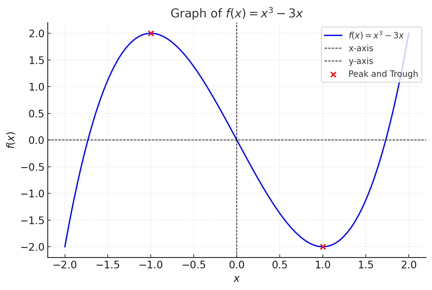
As you can tell, it has one peak (high point) and one trough (low point).

Often in machine learning we are working with high-dimensional versions of this problem and want to find the locations (the value of x) where the function value f(x) is at some extremum, either a high point (a maximum) or a low point (called a minimum). It is in fact finding these points that is the real goal of function optimization (training).

We can use the derivative to find these extremal points. Remember, the derivative of a function at a point tells us the rate of change of the change at that point. In graphical terms, it gives us a slope at that point. It is as if we pretend the function is made out of tiny little line segments (instead of a continuous curve) and then find the slope of the little line segment at the point we care about.

Here’s how we can find the extremal points:

1. Differentiate the function
   Start with f(x)=x3−3xf(x) = x³ − 3xf(x)=x3−3x.
   The derivative is:
   ∂f/∂x = 3x² − 3.

2. Set the derivative to zero
   Extremal points occur where ∂f/∂x = 0:
   3x² − 3 = 0.

3. Solve for x
   Simplify the equation:
   x² − 1 = 0
   x² = 1
   x = ±1.

4. Find the function values at critical points
   Substitute x = 1 and x = −1 into f(x):

   • For x = 1:
     f(1) = (1)³ − 3(1) = −2.

   • For x = −1:
     f(−1) = (−1)³ − 3(−1) = 2.

5. Peak: x = −1, f(−1) = 2

6. Trough: x = 1, f(1) = −2

Derivatives in higher dimenions

We can do the same thing for higher dimensional functions using the concept of a partial derivative.

Consider the function f(x,y) = x² + y². This is a function of two variables. We can only take the derivative of one variable at a time, so we call each one a partial derivative: ∂f/∂x and ∂f/∂y. Partial derivatives are no more difficult than regular derivatives; to take a partial derivative with respect to one variable, you just pretend the other variable is a constant number.

In this case, ∂f/∂x = 2x and ∂f/∂y = 2y.

Here’s the graph of this function:

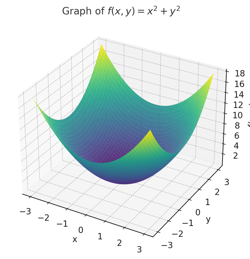
It’s shaped like a bowl, so in machine learning we would be interested in finding the point (x,y) where f(x,y) is at a minimum. We do this in the same way we did before: we find the (partial) derivatives and set them equal to 0, and solve for x and y.

• Set the Partial Derivatives to Zero
  To find the minimum, set both partial derivatives equal to 0:
  ∂f/∂x = 2x = 0
  ∂f/∂y = 2y = 0

• Solve for x and y
  From the equations:
  2x = 0 ⟹ x = 0
  2y = 0 ⟹ y = 0

So the point (x = 0, y = 0) is the minimum of this function.

Complex high-dimensional functions may have more than one minimum, and one minimum might be lower or higher than another. So we distinguish between local minima and global minima. The former are low points relative to their nearby points but are not the lowest points considering the whole function, whereas global minima are the lowest points across the whole function.

The Chain Rule

There is a whole bunch of procedures and tips and tricks on how to differentiate different kinds of functions. By remembering a few simple rules, you can easily differentiate most kinds of functions we care about in machine learning.

• Constant Rule:
  ∂/∂x(c) = 0
  (The derivative of a constant is always 0.)

• Power Rule:
  ∂/∂x(xⁿ) = n × xⁿ⁻¹
  (The derivative of x raised to the power of n.)

• Sum Rule:
  ∂/∂x(f(x) + g(x)) = ∂f/∂x + ∂g/∂x
  (The derivative of a sum is the sum of the derivatives.)

• Difference Rule:
  ∂/∂x(f(x) − g(x)) = ∂f/∂x − ∂g/∂x
  (The derivative of a difference is the difference of the derivatives.)

• Product Rule:
  ∂/∂x(f(x) × g(x)) = (∂f/∂x) × g(x) + f(x) × (∂g/∂x)
  (The derivative of a product of two functions.)

• Quotient Rule:
  ∂/∂x(f(x) ÷ g(x)) = [(∂f/∂x) × g(x) − f(x) × (∂g/∂x)] ÷ g(x)²
  (The derivative of a quotient of two functions.)

• Chain Rule:
  ∂/∂x(f(g(x))) = (∂f/∂g) × (∂g/∂x)
  (The derivative of a composition of functions.)

• Exponential Rule:
  ∂/∂x(eˣ) = eˣ
  (The derivative of the natural exponential function.)

• Logarithmic Rule:
  ∂/∂x(ln(x)) = 1/x
  (The derivative of the natural logarithm.)

• Constant Multiple Rule:
  ∂/∂x(c × f(x)) = c × (∂f/∂x)
  (The derivative of a constant multiplied by a function.)

I want to focus on the chain rule because this rule is critical for deep learning.

Consider a function like f(x) = (3x+1)². We can decompose this function into two separate functions.

g(u) = u² and h(x) = 3x + 1

Then we can re-phrase f(x) as f(x) = g(h(x)), because f(x) = (h(x))² = (3x + 1)²

The chain rule tells us that we can get the derivative of the original function f(x) by differentiating g(h(x)) and h(x) and simply multiplying their derivatives.

Which is the correct derivative.

Neural networks are functions that can be decomposed like this, and we can use the chain rule to differentiate them like this. We will need to do that in the future. For now, we continue to build up our foundational knowledge.

It turns out, we can use this new tool of differentiation to make a much better version of the iterative nudge training algorithm. As we discussed at the beginning, the nudge algorithm works but it doesn’t scale well to larger problems because it’s computational complexity is 𝒪(np²), where n is the number of data points and p is the number of parameters.

Instead, we can differentiate the mean absolute error (MAE) function, with respect to the parameter vector W, and that will tell us the exact rate of change of the MAE at a particular choice of W. So if we have a starting W, then we can use the derivative of the MAE to tell us which changes of W lead toward a smaller MAE.

It’s actually a bit complicated to a differentiate the MAE by hand, so instead of the MAE, let’s use a different, and in fact more common, error (objective) function called the mean squared error (MSE).

The inputs to the MSE are X (a list of data point vectors in the form of [year, CO₂]), y, (the list of ground truth labels), and W (the parameter vector). The yᵢ in this expression refer to the ground truth (“labels”) temperature anomalies and the Xᵢ ⋅ W part is the prediction from the model. So we take the difference between the true temperature anomaly and the predicted temperature anomaly and square the result, and do that for all the data points, sum all those squared errors together, and divide by the number of data points to get the average (mean) squared error.

The MSE expression looks similar in form to the f(x) = (3x+1)² function we differentiated with the chain rule earlier. We can apply the same principles. We want to get the derivative of the MSE with respect to the W parameter vector.

Here are the steps:

1. Recognize the Composition
   The MSE is a sum of squared terms, so we can apply the chain rule. Specifically:

   • Outer function: u(z) = z²

   • Inner function: h(X, y; W) = yᵢ − Xᵢ ⋅ W

   • Substituting into the MSE: MSE(X, y; W) = (1/n) Σᵢⁿ u(h(X, y; W)).

2. Differentiate the Outer Function (u(z))
   The derivative of u(z) = z² is: ∂u/∂z = 2z.

   So, for each term in the sum: (∂/∂W) u(h(X, y; W)) = 2 ⋅ h(X, y; W) ⋅ (∂/∂W) h(X, y; W).

3. Differentiate the Inner Function (h(X, y; W))
   The inner function is: h(X, y; W) = yᵢ − Xᵢ ⋅ W.

   The derivative with respect to W is: (∂/∂W) h(X, y; W) = −Xᵢ.

4. Combine Using the Chain Rule
   Substituting ∂u/∂z and ∂h/∂W into the chain rule: (∂/∂W) u(h(X, y; W)) = 2 ⋅ (yᵢ − Xᵢ ⋅ W) ⋅ (−Xᵢ).

   Simplify: (∂/∂W) u(h(X, y; W)) = −2 ⋅ (yᵢ − Xᵢ ⋅ W) ⋅ Xᵢ.

5. Sum Over All Data Points
   The MSE is the mean of all terms, so sum over all data points and divide by n: ∂MSE(X, y; W)/∂W = (1/n) Σᵢⁿ −2 ⋅ (yᵢ − Xᵢ ⋅ W) ⋅ Xᵢ.

   Simplify further: ∂MSE(X, y; W)/∂W = −(2/n) Σᵢⁿ (yᵢ − Xᵢ ⋅ W) ⋅ Xᵢ.

6. Final Answer
   The gradient of the MSE with respect to W is:

   ∂MSE(X, y; W)/∂W = −(2/n) Σᵢⁿ (yᵢ − Xᵢ ⋅ W) ⋅ Xᵢ.

Here’s what the MSE and its derivative look like in Python code:

import numpy as np
def mse(X, y, W):
    """
    Compute the Mean Squared Error (MSE).
    Parameters:
    - X: 2D numpy array of shape (n, p), input data.
    - y: 1D numpy array of shape (n,), ground truth labels.
    - W: 1D numpy array of shape (p,), parameter vector.
    Returns:
    - mse: Mean Squared Error (float).
    """
    n = len(y)  # Number of data points
    predictions = np.dot(X, W)  # Model predictions
    errors = y - predictions  # Residuals
    mse = np.sum(errors**2) / n  # Mean of squared residuals
    return mse
def mse_derivative(X, y, W):
    """
    Compute the gradient of the Mean Squared Error (MSE) with respect to W.
    Parameters:
    - X: 2D numpy array of shape (n, p), input data.
    - y: 1D numpy array of shape (n,), ground truth labels.
    - W: 1D numpy array of shape (p,), parameter vector.
    Returns:
    - gradient: 1D numpy array of shape (p,), gradient of MSE with respect to W.
    """
    n = len(y)  # Number of data points
    predictions = np.dot(X, W)  # Model predictions
    errors = y - predictions  # Residuals
    gradient = -2 / n * np.dot(X.T, errors)  # Gradient of MSE
    return gradient

The derivative of the MSE with respect to its parameters W, ∂MSE(X, y; W)/∂W, is also called the gradient of MSE, and is often denoted using the nabla symbol: ∇MSE(X, y; W).

The gradient of a function returns a vector of the partial derivatives of the function with respect to its parameters.

We are now finally ready to do gradient descent.

We want to minimize the error of the MSE with respect to its parameters, so we can do this:

wᵢ = wᵢ − η ⋅ ∇MSE(X, y; W)

The parameter η is called the learning rate. The learning rate is usually a small number like 0.01. The gradient of the MSE will tell us which direction the MSE is increasing or decreasing for a given W. So if ∇MSE(X, y; W) is negative for a given W, then that means the MSE is decreasing in that direction, so we should increase wᵢ to further minimize the error. Conversely, if ∇MSE(X,y;W) is positive for a given W, then the MSE is increasing in that direction, so we should decrease wᵢ. This is why gradient descent moves opposite to the direction of the gradient: to ensure the MSE gets smaller with each step.

The learning rate controls how big each step we take is. We iteratively increase or decrease the W parameters based on the gradient by a little bit until we find the minimum of the MSE with respect to W. At that point, the model has been trained or optimized.

Summary:

In this post, we explored the foundations of optimization in machine learning, specifically focusing on improving models using differentiation and gradient descent. Here's the key breakdown:

1. Iterative Nudge Algorithm:

   • Initially, we used a trial-and-error approach to adjust parameters by small amounts, but this method has a computational complexity of 𝒪(n⋅p²), making it inefficient for larger datasets and models.

2. From MAE to MSE:

   • To simplify differentiation, we shifted from the Mean Absolute Error (MAE) to the Mean Squared Error (MSE), which is easier to differentiate mathematically.

3. Using Derivatives:

   • We derived the gradient of the MSE with respect to model parameters WWW using the chain rule. The gradient ∇MSE(X,y;W) provides the exact direction to adjust W to minimize the error.

4. Gradient Descent:

   • Gradient descent replaces the inefficient nudge algorithm with an update rule:
     W = W − η⋅∇MSE(X,y;W), where η (the learning rate) controls the step size.

   • This algorithm is computationally efficient, scaling with 𝒪(n⋅p).

5. Derivatives and Optimization:

   • Derivatives help find critical points (minima, maxima) by indicating where the slope (rate of change) of a function is zero.

   • For 1D and 2D functions, we demonstrated how derivatives and partial derivatives can locate these extremal points.

6. Building Blocks for Neural Networks:

   • The chain rule and gradient descent are essential tools in machine learning, especially for training multi-layered neural networks by optimizing their parameters.

By leveraging these mathematical tools, we’ve established a strong foundation for optimization, which we’ll use to explore more complex models and algorithms in future posts.