DiffusionGemma Explained

Google recently released DiffusionGemma, a 26B open-weight uniform state diffusion language model ~4× faster than Gemma 4 for certain workloads.1

As an experimental model, it doesn’t have a whitepaper, and the officially released docs are pretty brief and high-level. This blog post, based on the colab notebook, attempts to fill in the gaps. It walks through an annotated from-scratch reimplementation derived from its open weights, following the style of the awesome Annotated Transformer.

Along the way, we explain some of the more opaque details — behind the model architecture, self-conditioning, the sampling procedure, how encode/decode weight sharing is actually implemented. Through closely examining the model config and weights, we also uncover some interesting design choices — the layer scalar, partial RoPE, and Google’s Scalar QK Norm — and offer possible explanations for them. Finally, we conclude by making some visualizations and empirical observations about the denoising process.

Thank you Lucas Gu, Arshia Nayebnazar, Henry Ko, Rishi Athavale, and Tejas Prabhune for help proofreading and improving this blog post!

Note: prior knowledge of vanilla autoregressive LLM implementation (Llama 3.1, MOE) is assumed.

• Setup + Load Model

  • Google’s Scalar QK Normalization

  • Rotary position embeddings

• Attention

  • Decode vs Encode

  • Gemma-specific details

  • Optimizations and Implementation

• MOE

  • MOE Forward

  • Routing Score

  • RMSNorm Fusion

• Putting Them together

  • Logit Softcapping

  • Denoise vs Prefill

  • Layer Scalar

• Sampling

  • Lazy Sampling

  • Stage Then Commit

  • Preliminary Analysis

• References

Install, import, load configs and weights

!pip install -q -U huggingface_hub
!hf download google/diffusiongemma-26B-A4B-it \
    --local-dir /content/diffusiongemma
import glob
import json
import torch
import torch.nn.functional as F
from einops import rearrange, einsum
from safetensors.torch import load_file
from tokenizers import Tokenizer
from torch.distributions import Categorical
from tqdm import trange
torch.set_default_device("cuda")
max_tot_tokens = 2048
checkpoint = "diffusiongemma"
canvas_len = 256
model_config = json.load(open(f"{checkpoint}/config.json"))['text_config']
gen_config = json.load(open(f"{checkpoint}/generation_config.json"))
V = model_config['vocab_size']
sd = {}
for safetensor_path in glob.glob(f"{checkpoint}/model-*.safetensors"):
    sd |= {k: v for k, v in load_file(safetensor_path, device="cuda").items() if "vision" not in k}
W_vocab = sd['model.decoder.embed_tokens.weight']
sd

Printing out the weights, we find that interestingly, all entries within each learned QK-normalization weight vector have the same value. For example:

'model.decoder.layers.17.self_attn.q_norm.weight': tensor(
    [0.9883, 0.9883, 0.9883, 0.9883, 0.9883, 0.9883, 0.9883, 0.9883,
     0.9883, 0.9883, 0.9883, 0.9883, 0.9883, 0.9883, 0.9883, ...]
)

The QK-norm weight vectors have the form

where γ_q and γ_k are the learned scalars.

RoPE preserves Euclidean norm, so the same result holds after applying rotate:

For a query q and key k_i separated by an angle θ_i,

Thus, the attention score for k_i is

where

is a fixed, learned effective attention temperature per layer.

In regular QK norm models (and non-QK norm models), the magnitudes of q and k can vary. This 1) produces a per-query-dependent effective temperature and 2) allows key magnitude to encode a form of query-independent “global importance”:

This may be undesirable in long-context settings, where a high-magnitude early key could remain disproportionately influential even after its relevance has faded. One interpretation is that scalar QK norm effectively avoids this, and makes the inner product truly capture similarity between a q and k without being confounded with anything else.

Verify all QK norm weights are like this

for layer_id in range(model_config["num_hidden_layers"]):
    for kind in ("q", "k"):
        w = sd[f"model.decoder.layers.{layer_id}.self_attn.{kind}_norm.weight"]
        assert (w == w[0]).all(), "QK Norm entries are not all equal"

We do RMSNorm in higher precision like usual because precision errors are accumulated through the reduction, potentially amplified through the division, and propagated to every element.

RMSNorm

def rms(x, w = 1):
    return (w * x * (x.shape[-1] ** 0.5) / (torch.norm(x, dim=-1, keepdim=True, dtype=torch.float32) + model_config['rms_norm_eps'])).to(x.dtype)

DiffusionGemma has two RoPE configs:

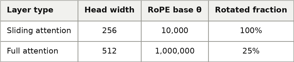
Standard RoPE assigns each of the d/2 complex / rotary pairs one frequency (head dim d):

This is what the sliding-attention layers use, but interestingly, DiffusionGemma’s full-attention layers use partial RoPE: after constructing the normal frequency vector, we then set all but the first 25% of its pair frequencies to zero, which will make rotate a no-op on those dimensions. Notably, we are doing truncating the full frequency spectrum, not the more intuitive option of rescaling it similar to YaRN and other long-context extension methods.

Partial RoPE enables a head to carry both explicitly position-sensitive features and features whose representation is not rotated as position changes.

Interestingly, the rows of W_k and W_q are stored arranged so that the projected vectors use split-half rotary pairs, (t, t + d/2), rather than adjacent pairs, (t, t+1), as in the original RoFormer paper. This makes the rotation easier to express and slightly more cache-friendly.

From equation 34 in RoFormer,

where rot(x) rotates each two-dimensional pair by 90 degrees counterclockwise, thus for a token at position p, the i-th pair of its k/q vector is rotated ccw by ω_i * p. Note our code’s rotate(x) is RoPE(x), not to be confused with rot(x).

In other words, instead of something like

rot_x = np.empty_like(x)
rot_x[..., 0::2] = -x[..., 1::2]
rot_x[..., 1::2] =  x[..., 0::2]

for (t, t+1) pairs,

we have the more cache friendly

rot_x = rearrange([-x[..., head_dim // 2 :], x[..., : head_dim // 2]], 'z ... d -> ... (z d)')

Precompute RoPE frequencies and rotate

# precompute frequencies
freq = {}
# sliding window - regular rope
freq['sliding_attention'] = model_config['rope_parameters']['sliding_attention']['rope_theta'] ** -(torch.arange(0, 1, 2 / model_config['head_dim'], dtype=torch.float32))
# full attention - partial rope
freq['full_attention'] = model_config['rope_parameters']['full_attention']['rope_theta'] ** -(torch.arange(0, 1, 2 / model_config['global_head_dim'], dtype=torch.float32))
freq['full_attention'][int(model_config['rope_parameters']['full_attention']['partial_rotary_factor'] * len(freq['full_attention'])) : ] = 0
def rotate(x, layer_type, start_idx=0): # x [..., seq, head_dim]; rotate each (t, t + hd/2) pair ccw
    head_dim = x.shape[-1]
    rot_x = rearrange([-x[..., head_dim // 2 :], x[..., : head_dim // 2]], 'z ... d -> ... (z d)')
    pos = (torch.arange(x.shape[-2])[:, None] + start_idx) * torch.cat([freq[layer_type], freq[layer_type]]) # pos * (t, t + hd/2 pairs)
    return torch.cos(pos).to(x.dtype) * x + torch.sin(pos).to(x.dtype) * rot_x

In the decode stage, each canvas query attends to [committed history | current canvas]. It is:

• Similar to autoregressive prefill in the sense that it writes KV’s for several tokens at a time, autoregressive decode in the sense that it reads a context history of past KV’s

• Similar to cross attention in that it attends to KV’s from the encoder, whisper-style, similar to self-attention in that it is non-casual, ViT-style

In the encode stage, the attention behaves like an ordinary causal prefill. It can be thought of as the “verify” pass for speculative decoding with a 256-token draft, with all tokens accepted.

The same exact attention weights is used for both.

This code can be easily modified to support batch size greater than 1, but it does not support mixed encode/decode modes within the same batch. Dynamic per-sequence attention mode is supported in vLLM:

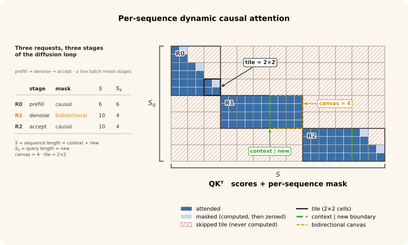
Here, “denoise” means decode, “prefill” means encode on the prompt, and “accept” means encode on a denoised canvas.

For sliding layers, we use the approach in Google DeepMind’s JAX sampler: every canvas token sees all other tokens inside the canvas plus the same prefix of KVs immediately before the canvas. Note that vLLM uses a different symmetric, 2K+1, per-token sliding window.

Some notable differences from a standard LLM attention:

1. No explicit 1/√d multiplier. The inner product is done directly. This can absorbed into the scalar Q/K normalization weights, which already does a fixed inverse temperature.

2. Gemma also applies an embedding scale, multiplying token embeddings by √D at the start of the residual stream. I’m not really sure why this is done.

3. Value normalization. Weightless RMS-norm (i.e., unit norm) is applied to every value vector before it is used or stored in cache

4. Hybrid architecture. 5 : 1 ratio of sliding window layers to global attention layer

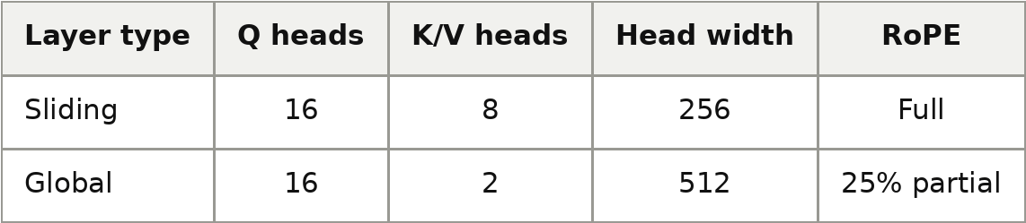
5. Shared global K/V projection. In full-attention layers, W_v = W_k. K and V are only different due to post-projection processing: K receives scalar-weight RMS normalization plus RoPE, while V receives unit RMS normalization and no RoPE. This is strange since K/V vectors are typically believed to live in different subspaces (see 1, 2 while K/Q live in the same subspace).

One potential optimization is to cache only the shared pre-normalization projection and reconstruct K and V when reading it, potentially reducing global-layer cache storage at the cost of additional computation. Combined with the hybrid global/sliding schedule, this could be attractive in long-context, KV-cache-bandwidth-bound regimes. The readable implementation below keeps separate K and V caches instead.

One implemented optimization is that, on encode, we can skip all computation after the K/V projection in the final layer, skipping most of the final layer and unembed work. Encode passes do not use the model’s final logits; they only need to incur the minimum set of computation required to obtain (and commit) correct K/V states in every layer.

In the current implementation with fixed-size statically-shaped cache, full-attention is only differentiated from sliding window through kv_len, thus behaves exactly like sliding-window attention with a max_tot_tokens-sized window:

class AttentionBlock(torch.nn.Module):
    def __init__(self, layer_id):
        super().__init__()
        self.layer_id = layer_id
        self.layer_type = model_config['layer_types'][layer_id]
        self.W_q, self.W_k, self.W_o = [sd[f'model.decoder.layers.{layer_id}.self_attn.{item}_proj.weight'] for item in ['q', 'k', 'o']]
        self.q_norm, self.k_norm = [sd[f'model.decoder.layers.{layer_id}.self_attn.{item}_norm.weight'] for item in ['q', 'k']]
        self.pre_norm = sd[f'model.decoder.layers.{layer_id}.input_layernorm.weight']
        self.post_norm = sd[f'model.decoder.layers.{layer_id}.post_attention_layernorm.weight']
        self.q_heads = model_config['num_attention_heads']
        if self.layer_type == 'full_attention':
            self.W_v = self.W_k # global layers share K = V
            self.kv_heads = model_config['num_global_key_value_heads']
            self.head_dim = model_config['global_head_dim']
            self.kv_len = max_tot_tokens
        else:
            assert(self.layer_type == 'sliding_attention')
            self.W_v = sd[f'model.decoder.layers.{layer_id}.self_attn.v_proj.weight']
            self.kv_heads = model_config['num_key_value_heads']
            self.head_dim = model_config['head_dim']
            self.kv_len = model_config['sliding_window']
        self.k_cache = torch.empty(self.kv_heads, self.kv_len, self.head_dim) # use statically shaped KV buffer
        self.v_cache = torch.empty(self.kv_heads, self.kv_len, self.head_dim) # KV's flow into here from left to right, FIFO, latest element is rightmost
    def forward(self, x, pos_idx, mode):
        assert mode in ['encode', 'decode']
        L, D = x.shape
        resid_x = x.clone()
        x = rms(x, w=self.pre_norm)
        q, k, v = x @ self.W_q.T, x @ self.W_k.T, x @ self.W_v.T
        q, k, v = [rearrange(z, 'l (n h) -> n l h', h = self.head_dim) for z in [q, k, v]]
        q, k = rms(q, self.q_norm), rms(k, self.k_norm) # QK-norm per head: weight is [head_dim], normalize over each head's dims
        v = rms(v, 1) # v_norm: weightless, no rope
        q, k = rotate(q, self.layer_type, pos_idx), rotate(k, self.layer_type, pos_idx) # absolute positions pos_idx .. pos_idx + L
        k = torch.concat([self.k_cache[:, : pos_idx, :], k], axis=1) # attend to [committed history | current block]
        v = torch.concat([self.v_cache[:, : pos_idx, :], v], axis=1) # Note python automatically clips on the left to 0, on the right to shape[1] = kv_len
        if mode == "encode": # difference #1: writes/updates the kv cache
            # Actually, we don't have to put this in a branch, can also just do this on decode too, ok since we'll override with an encode at the end anyways
            self.k_cache[:, : pos_idx + L, :] = k[:, -self.kv_len :, :] # automatically clips
            self.v_cache[:, : pos_idx + L, :] = v[:, -self.kv_len :, :]
            if self.layer_id == model_config['num_hidden_layers'] - 1:
                return # encode optimization: notice we don't need to do the remaining computation after this
        q = rearrange(q, '(n gqa) qt h -> n gqa qt h', gqa = self.q_heads // self.kv_heads) # Fold GQA into an outer dim
        scores = einsum(q, k, 'n gqa qt h, n kt h -> n gqa qt kt').float() # no divide by sqrt(head dim); softmax in fp32
        if mode == "encode":
            scores += torch.triu(torch.full(scores.shape, -torch.inf), diagonal = scores.shape[-1] - scores.shape[-2] + 1) # this applies a mask that looks like R2 in the vllm figure
        scores = torch.exp(scores - torch.amax(scores, axis=-1, keepdims=True))
        scores = (scores / torch.sum(scores, axis=-1, keepdims=True)).to(x.dtype)
        x = einsum(scores, v, 'n gqa qt kt, n kt h -> n gqa qt h')
        x = rearrange(x, 'n gqa qt h -> qt (n gqa h)')
        res = x @ self.W_o.T
        res = rms(res, self.post_norm)
        return res + resid_x

DiffusionGemma routes each token to 8 of 128 experts + one larger shared expert per forward pass.

Each expert is a standard gated GELU MLP:

HuggingFace stores the routed experts’ gate and up projections as a single matrix, which we explicitly split in the MLP module.

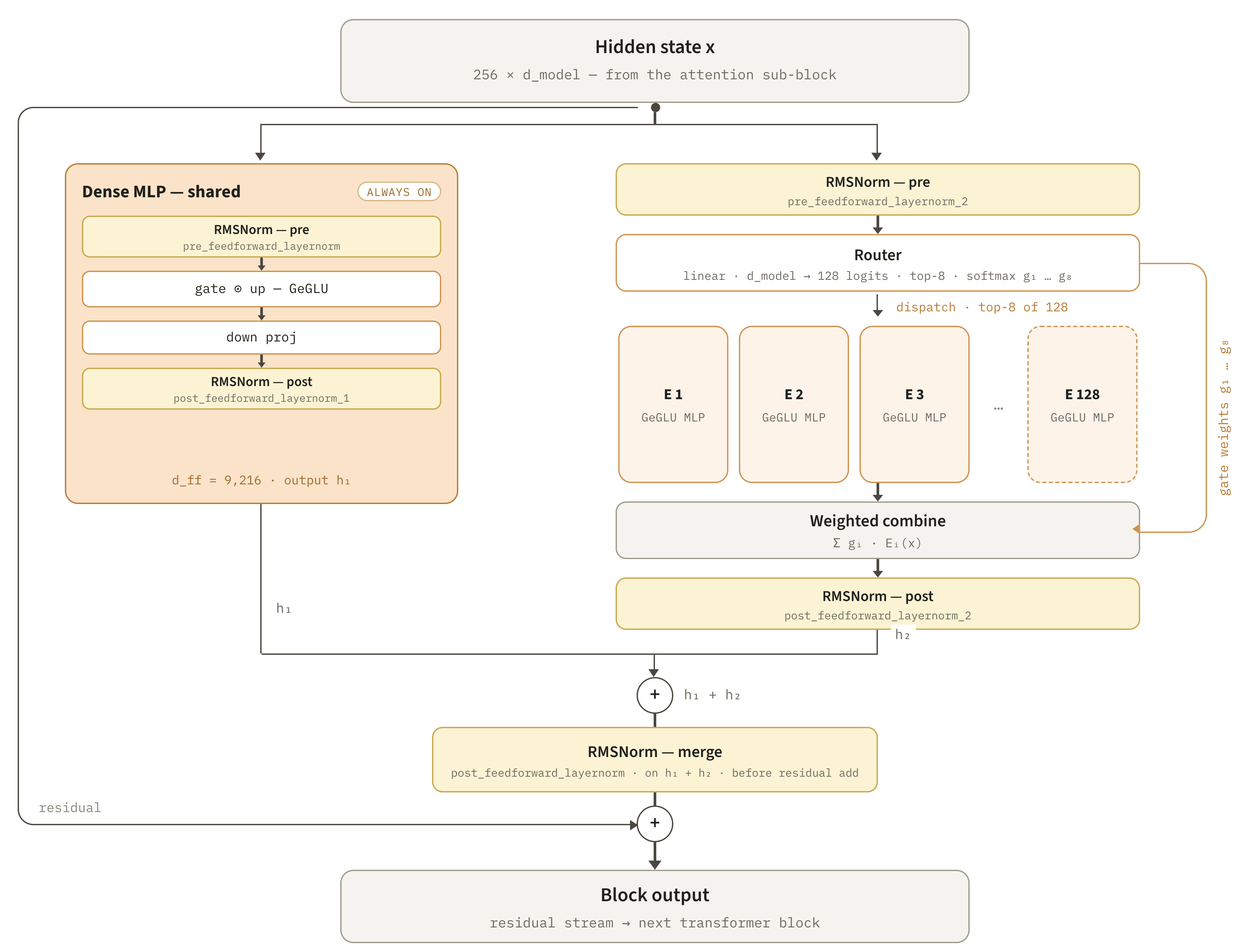
operates independently across the token axis. Each (of B × L many tokens) is routed to its own 8 experts. We could do this naively by looping over each token, but a better approach is to iterate over the experts instead: gather all tokens routed to each expert, do a single forward pass, then send results back.

Across multiple devices / for expert parallelism, this is usually implemented with an AllToAll-style collective rather than the slow explicit Python loop we have here (see the JAX Scaling Book).

DiffusionGemma performs routing in the standard way. Each expert receives a score proportional to

where the expert keys are the rows of W_router. The top 8 scores are renormalized and multiplied by learned per-expert scales.

There is an optimization we can do here to save a couple RMS-norm computations. Notice that we apply a pre-norm 1 (shared expert) + 8 (routed experts) times at the start of each MLP. Notice RMSNorm can be factored into two operations

, unit-normalize then multiply by w.

Instead of doing this naively, we can instead apply a single weightless RMS_1(x) at the start, and absorb each expert’s learned RMSNorm weight w into the columns of that expert’s gate and up projection matrix.

MLP and mixture-of-experts block

class MLP(torch.nn.Module):
    def __init__(self, layer_id, expert_num, conditioning_mlp : bool = False):
        super().__init__()
        if(conditioning_mlp):
            self.pre_norm = sd['model.decoder.self_conditioning.pre_norm.weight']
            self.W_up = sd['model.decoder.self_conditioning.up_proj.weight']
            self.W_gate = sd['model.decoder.self_conditioning.gate_proj.weight']
            self.W_down = sd['model.decoder.self_conditioning.down_proj.weight']
            return
        if expert_num is None:
            self.pre_norm = sd[f'model.decoder.layers.{layer_id}.pre_feedforward_layernorm.weight']
            self.W_up, self.W_gate, self.W_down = [sd[f'model.decoder.layers.{layer_id}.mlp.{item}_proj.weight'] for item in ['up', 'gate', 'down']]
        else:
            self.pre_norm = sd[f'model.decoder.layers.{layer_id}.pre_feedforward_layernorm_2.weight']
            self.W_gate, self.W_up = rearrange(sd[f'model.decoder.layers.{layer_id}.experts.gate_up_proj'][expert_num], '(z intermed) D -> z intermed D', z=2)
            self.W_down = sd[f'model.decoder.layers.{layer_id}.experts.down_proj'][expert_num]
    def forward(self, x): # every MLP has a prenorm. Also, note since the MLP is a compsition of functions that maps the 0 vector to itself, the entire MLP also maps all 0s to all 0s, this is relevant for the self-conditioning MLP
        L, D = x.shape
        x = rms(x, self.pre_norm)
        a = x @ self.W_up.T
        b = F.gelu(x @ self.W_gate.T)
        res = (a * b) @ self.W_down.T
        assert(res.shape == (L, D)) # share expert, routed expert, and self-conditioning MLP all map (_, D) -> (_, D)
        return res
class MOEBlock(torch.nn.Module):
    def __init__(self, layer_id):
        super().__init__()
        self.k_experts = model_config['top_k_experts']
        self.num_experts = model_config['num_experts']
        self.W_router = sd[f'model.decoder.layers.{layer_id}.router.proj.weight']
        self.expert_scale = sd[f'model.decoder.layers.{layer_id}.router.per_expert_scale']
        self.scale = sd[f'model.decoder.layers.{layer_id}.router.scale']
        self.experts = [MLP(layer_id, e) for e in range(self.num_experts)]
        self.shared_expert = MLP(layer_id, None)
        self.post_norm_1 = sd[f'model.decoder.layers.{layer_id}.post_feedforward_layernorm_1.weight'] # applied on shared expert output
        self.post_norm_2 = sd[f'model.decoder.layers.{layer_id}.post_feedforward_layernorm_2.weight'] # applied on summed contribution from experts
        self.post_norm = sd[f'model.decoder.layers.{layer_id}.post_feedforward_layernorm.weight'] # the sum h1 (shared ) + h2 (routed sum), before residual add
    def forward(self, x):
        L, D = x.shape
        resid_x = x.clone()
        route_x = rms(x) * self.scale / (D ** 0.5)
        expert_scores = F.softmax((route_x @ self.W_router.T).float(), dim=-1) # (L, num_experts)
        top_k_scores, top_k_idx = torch.topk(expert_scores, self.k_experts, dim=-1) # (L, k_experts), (L, k_experts)
        top_k_scores = (top_k_scores / torch.sum(top_k_scores, dim=-1, keepdim=True) * self.expert_scale[top_k_idx]).to(x.dtype)
        res = rms(self.shared_expert(x), self.post_norm_1) # h1: dense branch, shape (L, D)
        moe_out = torch.zeros_like(x)
        for id, expert in zip(range(self.num_experts), self.experts):
            mask = torch.any(top_k_idx == id, dim = -1) # boolean mask (L, ) which tokens routed to expert_id
            mult = top_k_scores[mask][top_k_idx[mask] == id] # shape (L', ) where L' <= L is the number of tokens expert_id routed to
            moe_out[mask] += mult[:, None] * expert(x[mask]) # (L', D) += (L', 1) * (L', D)
        res = res + rms(moe_out, self.post_norm_2) # h2 normed once, then h1 + h2
        return rms(res, self.post_norm) + resid_x

We now combine all our previous components into a single module. Unlike Llama, DiffusionGemma does a couple things different beyond merely interleaving attention and MoE blocks.

Logit softcapping applies the following function to the final logits:

where z is an uncapped logit and c is the softcap value.

For |z| ≪ c, tanh(z/c) ≈ z/c, so small logits are essentially unchanged. As z → ±∞, z_capped → ± c, so large logits are “soft-capped”.

This is a smooth alternative to torch.clip or torch.clamp - unlike a hard cap, it remains differentiable everywhere.

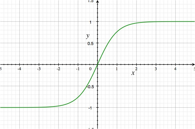
The standard tanh function is bounded between -1 and 1; multiplying by c changes the bounds to [−c,c].

Note this is part of the model, and not the sampling process — not to be confused with the temperature schedule, which is applied later.

The following are function signatures of encode vs decode:

# this commits canvas, (last time we) write KV cache
def enc(self, pos_idx, logits) -> None:
    self._forward(pos_idx, logits, 0, mode="encode")
# this maps (canvas_i, canvas_prob_i) -> (canvas_prob_i+1)
def dec(self, pos_idx, logits, logit_probs) -> torch.tensor:
    return self._forward(pos_idx, logits, logit_probs, mode="decode")

On encode, the embedded tokens are directly passed into the first layer.

In decode mode, the embedded tokens additionally incorporates a self-conditioning signal from the previous denoising step. Let P∈ℝ^(L×V) be the previous step’s post-softmax probability distribution over vocabs at each of L canvas positions, let E∈ℝ^(V×D) be the tied embedding table. Then, P @ E computes the expected token embeddings from the previous iteration, L independent convex sums with the weights stored in P. This is then passed through a small conditioning MLP, added to the canvas token embedding, and RMSNormed. Self-conditioning is helpful because for example,

• Knowing how confident the previous pass was in this token can inform us about how confident we should be in this pass

• During sampling, the highest entropy, least confident tokens are replaced by a random token ID. Thus, self-conditioning allows the model to deduce which tokens are effectively [MASK] tokens by comparing the probability distribution input to the token input. 2

• Possibly gives a way for gradients to flow across denoising steps

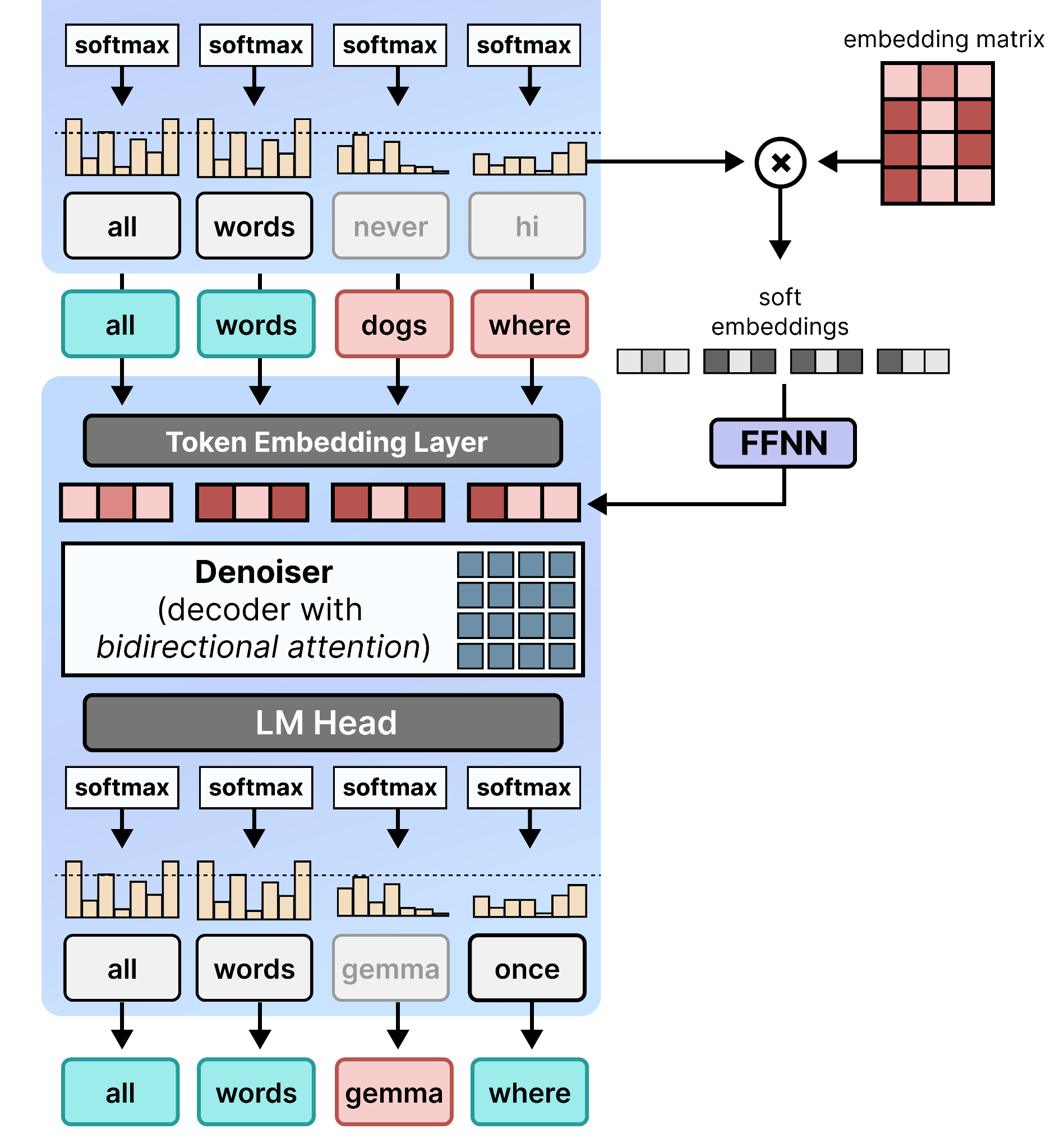
On the first decode step, the self-conditioning input is all 0s. Note that since the self-conditioning MLP is composed of functions that map all 0s to all 0s, the added contribution from self-conditioning to the input is 0 - this is equivalent to skipping self-conditioning for that step (no previous “self”).

Notice each block of computation in DiffusionGemma is additive to the residual stream:

where F is the core computation in that block, and RMSNorm(x) is that block’s pre-norm (both attention and MOE have this).

Thus due to the skip connections, the residual stream remains unnormalized through all 30 layers. This is perfectly fine if the activations truly live in ℝ^n, but unfortunately, they are bound to the subset of representation values of its datatype, which has a fixed dynamic range - upper and lower bounds of the feasible set, and anything outside will over/underflow to infinities. To ensure this doesn’t happen, quantization methods typically multiply by a scalar S before casting, for example:

where

to ensure values lie within the dynamic range [−V_max, V_max].

A similar worry arises for the unnormalized residual stream, the magnitude of the activations may gradually grow through the layers (note however, the inputs to blocks remain well-conditioned due to the RMSNorm). To improve training stability, avoid overflow, and enable stable low-precision inference, DiffusionGemma adds a layer scalar which rescales the completed residual stream by a learned scalar s_l at the end of every layer:

Printing out the layer scalars’ actual values, we see that they are all < 1, which makes sense according to our interpretation. Interestingly, it is a learned parameter — the model could learn to adaptively regulate the magnitude of its own residual stream throughout training.

Notice the RMSNorm is invariant to multiplying its input by a scalar (RMSNorm(cx) = RMSNorm(x)). Since every block receives input through an RMSNorm, the layer scaler has little benefit on the normalized input presented to each block. However, note it will affect the direction of the input after the first layer.

The released Hugging Face checkpoint stores separate encoder and decoder layer-scalar entries,

sd[f"model.encoder.language_model.layers.{i}.layer_scalar"]
and
sd[f"model.decoder.layers.{i}.layer_scalar"]

but their values are actually identical. In the code below, we have a single self.layer_scalar.

Complete DiffusionGemma model

class DiffusionGemma(torch.nn.Module): # Any computation that utilizes parameters passes through here
    def __init__(self):
        super().__init__()
        self.W_embed = sd['model.decoder.embed_tokens.weight'] # also used as the unembedding matrix (tie_word_embeddings = True)
        self.attn_blocks = [AttentionBlock(i) for i in range(model_config['num_hidden_layers'])]
        self.moe_blocks = [MOEBlock(i) for i in range(model_config['num_hidden_layers'])]
        self.layer_scalar = [sd[f'model.encoder.language_model.layers.{i}.layer_scalar'] for i in range(model_config['num_hidden_layers'])]
        self.model_norm = sd['model.decoder.norm.weight'] # final / model norm
        self.embed_scale = torch.tensor(model_config['hidden_size'] ** 0.5)
        self.conditioning_MLP = MLP(layer_id=None, expert_num=None, conditioning_mlp=True)
    def _forward(self, pos_idx, logits, logit_probs, mode): # logit_probs = 0 <=> skip this path (no bias term anywhere)
        x = self.W_embed[logits] * self.embed_scale # (L, ) -> (L, D)
        # do self conditioning if decode
        if mode == "decode":
            condition_x = (logit_probs.to(x.dtype) @ self.W_embed) * self.embed_scale # (L, V) x (V, D) -> convex combination of vocab embeddings
            condition_x = self.conditioning_MLP(condition_x)
            x = rms(x + condition_x)
        # pass through all layers
        for i, (attn, moe) in enumerate(zip(self.attn_blocks, self.moe_blocks)):
            x = attn(x, pos_idx, mode)
            if x is None: # last encode layer wrote its KV cache and returned early; nothing else is needed
                return None
            x = moe(x)
            x = x * (self.layer_scalar)[i] # per-layer encoder/decoder scalar
        x = rms(x, self.model_norm)
        final_logits = (x @ self.W_embed.T).float() # (L, D) x (D, V) -> (L, V)
        return torch.tanh(final_logits / model_config['final_logit_softcapping']) * model_config['final_logit_softcapping']
    # this commits canvas, (last time we) write KV cache
    def enc(self, pos_idx, logits) -> None:
        self._forward(pos_idx, logits, 0, mode="encode")
    # this maps (canvas_i, canvas_prob_i) -> (canvas_prob_i+1)
    def dec(self, pos_idx, logits, logit_probs) -> torch.tensor:
        return self._forward(pos_idx, logits, logit_probs, mode="decode")

The following figure is a nice summary of what we’ve put together:

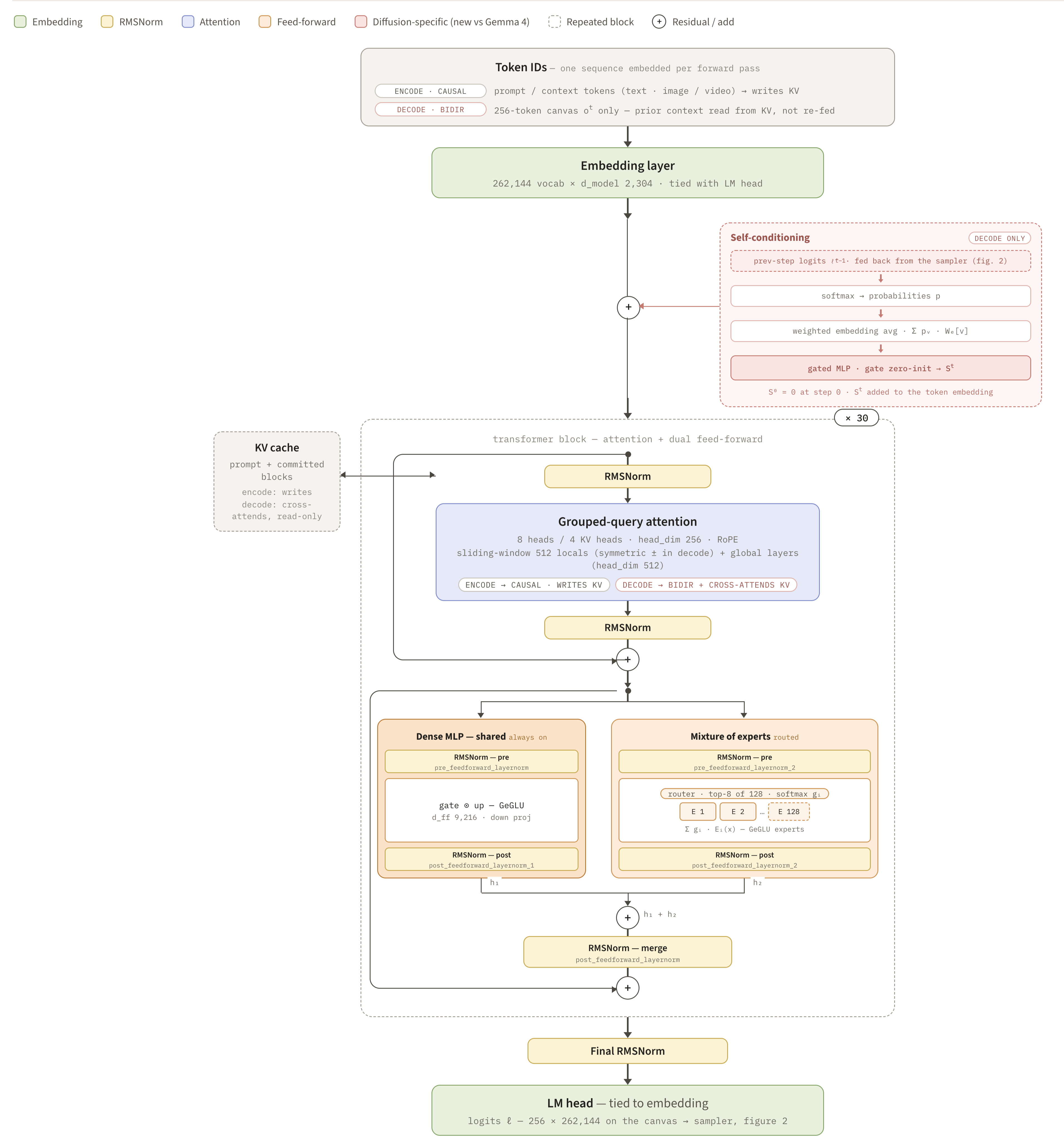
After the first encode on the input prompt, every 256 canvas of tokens incurs one encode pass and at most max_denoising_steps decode passes.

After obtaining a vocabulary distribution for every canvas position, sampling is more involved than in an autoregressive model.

We follow the sampling procedure explained here, implemented here. The meanings of the sampling parameters are documented here:

1. Apply temperature

   For decode pass i out of N = max_denoising_steps,

   \(t_i = t_{\max} + \frac{i}{N}\left(t_{\min}-t_{\max}\right), \qquad i=0,\ldots,N-1\)

   Thus the temperature starts at t_max and decreases toward t_min, increasingly sharpening the distribution. In the i-th iteration, we work with the categorical distribution formed by logits / t_i.

2. Compute entropy

   For every canvas position, we compute from its categorical distribution p,

   \(H(p) = -\sum_{v=1}^{V} p_v\log p_v\)

   Used as a measure of how uncertain the model is about the token at this position.

3. Keep a low-entropy prefix and renoise the rest

   Sort position entropies so that

   \(H_{(1)} \le H_{(2)} \le \cdots \le H_{(L)}\)

   Accept the largest prefix ending at k such that

   \(\sum_{j=1}^{k-1} H_{(j)} \le \texttt{entropy_bound}\)

   Then, replace every unaccepted position by a token drawn uniformly from the vocabulary.

4. Check for early stopping

   Convergence is decided when the canvas is confident and stable:

   • the argmax canvas has remained unchanged for stability_threshold (equals 1 here) previous canvases, and

   • the current canvas mean per-position entropy is below confidence_threshold.

On convergence or after N steps, we commit the latest canvas.

Tokenizer and sampling configuration

tok = Tokenizer.from_file(f"{checkpoint}/tokenizer.json")
prompt = """
What is the meaning of 67?
"""
chat = f"<bos><|turn>user\n{prompt}<turn|>\n<|turn>model\n"
max_denoising_steps = gen_config['max_denoising_steps'] # decoder forward passes per canvas
entropy_bound = gen_config['sampler_config']['entropy_bound'] # see formula in figure
t_max, t_min = gen_config['t_max'], gen_config['t_min'] # linear schedule of temperatures t_max -> t_min across the steps
confidence_threshold = gen_config['confidence_threshold']  # early-stop a canvas when argmax is stable (equal previous argmax canvas) and mean entropy < this
tokens = torch.tensor(tok.encode(chat, add_special_tokens=False).ids)
model = DiffusionGemma()

The usual way a denoising iteration is implemented:

Model forward → retain distribution for self-conditioning → sample and renoise tokens

Instead, we do sampling lazily, passing only the categorical distribution between steps and sampling only once we need it:

Stored distribution → sample and renoise input tokens → model forward → new distribution

The input into the first iteration is just all identical logits, which will generate a random canvas for us.

This is nice since:

• The only information we need to pass between steps is the self-conditioning input

• Initialization falls out naturally from a uniform categorical distribution, can be folded into the first step

• We can think of the decoder input as the previous canvas probs plus a source of randomness (from the sampling). Under this view, preparing the inputs (sampling) lazily is optimal. Additionally, it suggests an alternative interpretation of self-conditioning as the primary rather than auxiliary input:

One way to think of the decoder is that it repeatedly transports our current distribution toward the target distribution, reminiscent of a flow-like process on the probability simplex. So one can think about an alternate DiffusionGemma design that instead starts from a random position in the simplex at initialization, Categorical(probs=torch.rand(L, V)) or Categorical(logits=torch.rand(L, V)), rather than “Categorical(logits=torch.zeros(L, V))”.

We also intentionally give general functions for denoise which generates staged tokens; and commit, which takes in some staged tokens, generates their encoded KVs, and writes them to cache.

denoise(pos_idx) repeatedly calls decode against the already committed cache[:pos_idx] on a fresh canvas at positions [pos_idx : pos_idx + 256], and returns staged tokens sampled from the final canvas of logits. This function has no side effects on the KV cache, thus we can for example denoise multiple canvases at the same position and choose the best one. We can also place the canvas anywhere, as long as pos_idx ≤ len(tokens) - canvas_len, since the correct slice of the KV cache will automatically be read.

commit(l, r, staged_tokens) applies the casual encode and writes (or overwrites) the slice of KV cache from l to r, with the staged tokens’ KVs. This function allows arbitrary-lengthed blocks, thus we can for example commit only a confident prefix of the current canvas. We can also commit tokens at any positions, but if an earlier region is overwritten, all later tokens are invalidated because their cached states depended on the old prefix.

This design is to make alternative schedules easier to study, including overlapping canvases, revising an earlier block, selecting among several denoised candidates, or advancing only part of a canvas.

Denoise, stage, commit, and generate

def denoise(pos_idx): # returns staged_tokens
    assert pos_idx + canvas_len <= len(tokens) # must be length canvas_len (what if it wasn't fixed? analyze how casual the self attention is)
    plotting_data = []
    t = t_max
    t_step = (t_min - t_max) / max_denoising_steps
    last_canvas = Categorical(logits = torch.ones((canvas_len, V)))
    for step in trange(max_denoising_steps):
        # renoise last_canvas
        sH, sidx = last_canvas.entropy().sort(-1)
        accepted = torch.zeros_like(sH, dtype=torch.bool).scatter(-1, sidx, sH.cumsum(-1) - sH <= entropy_bound)
        last_canvas_noised = torch.where(accepted, last_canvas.sample(), torch.randint(0, V, (canvas_len,)))
        # pass in the noised tokens, but un-noised normalized probs (all-zero probs on step 0: the conditioning path maps 0 to 0)
        canvas = model.dec(pos_idx, last_canvas_noised, last_canvas.probs if step != 0 else torch.zeros(canvas_len, V)) / t; plotting_data.append(canvas.detach().cpu())
        canvas = Categorical(logits = canvas)
        if torch.mean(canvas.entropy()) < confidence_threshold and (canvas.logits.argmax(dim=-1) == last_canvas.logits.argmax(dim=-1)).all():
            return canvas.sample(), plotting_data
        t += t_step
        last_canvas = canvas
    assert False, f"Denoising not finished after {max_denoising_steps} steps"
def commit(l, r, staged_tokens):
    global tokens
    assert len(staged_tokens) == r - l + 1
    if(r + 1 < len(tokens)): # commits staged_tokens
        print(f"Invalidating {len(tokens) - (r+1)} tokens")
        tokens = tokens[:r+1]
    tokens[l:] = staged_tokens
    model.enc(l, staged_tokens)
def new_canvas():
    global tokens
    if len(tokens) + canvas_len > max_tot_tokens:
        return False
    nxt = torch.randint(V, (canvas_len,))
    tokens = torch.concat([tokens, nxt])
    return True
commit(0, len(tokens) - 1, tokens) # prefill: encode the chat prompt into the KV cache
pos_idx = len(tokens)
plotting_data = []
while new_canvas():
    staged_tokens, cur_data = denoise(pos_idx)
    commit(pos_idx, pos_idx + canvas_len - 1, staged_tokens)
    pos_idx = len(tokens)
    print('=' * 50)
    print('Final Canvas')
    print(tok.decode(tokens.tolist()))
    print('=' * 50)
    plotting_data.append(cur_data)
    if torch.isin(staged_tokens, torch.tensor(gen_config['eos_token_id'])).any():
        break

Output:

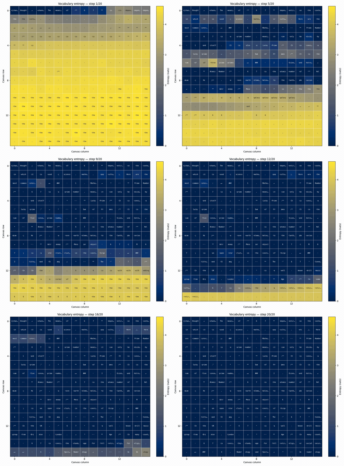
Using the saved plotting_data from denoise, we can make some figures of the denoising process over time:

Note the cells are laid out in reading order.

Without being explicitly trained to do so, it appears the model is approximately finalizing canvas tokens from left to right. Plotting two more figures:

Further confirms our suspicions.

At every step, the model seems to mostly focus its efforts on figuring out the next causal rolling window of tokens — it “thinks” casually. Is this a general behavior the model has learned? Let’s try a different prompt, solving a magic square puzzle:

Canvas 2

Canvas 3, More visualizations available here.

Interestingly, the prose tokens seem to exhibit the same causal pattern, but the magic square tokens do not. This makes intuitive sense. When humans solve these puzzles, the next value that’s easiest to deduce is not necessarily the next one in autoregressive order. This motivates perhaps a better explanation for how DiffusionGemma “thinks” during denoising — the “easiest”, lowest-entropy tokens are fixed / finalized / accepted first, which in turn unlocks / makes other tokens “easier” for the next denoising step. 3

Note this mirrors what we do during sampling: all but a prefix of lowest entropy tokens is renoised. For prose and chain-of-thought reasoning, the easiest tokens to resolve next often coincide with the earliest tokens in autoregressive order.

However for both prompts, once a token is accepted (i.e. low-entropy and not renoised), it’s extremely unlikely to be renoised in the future:

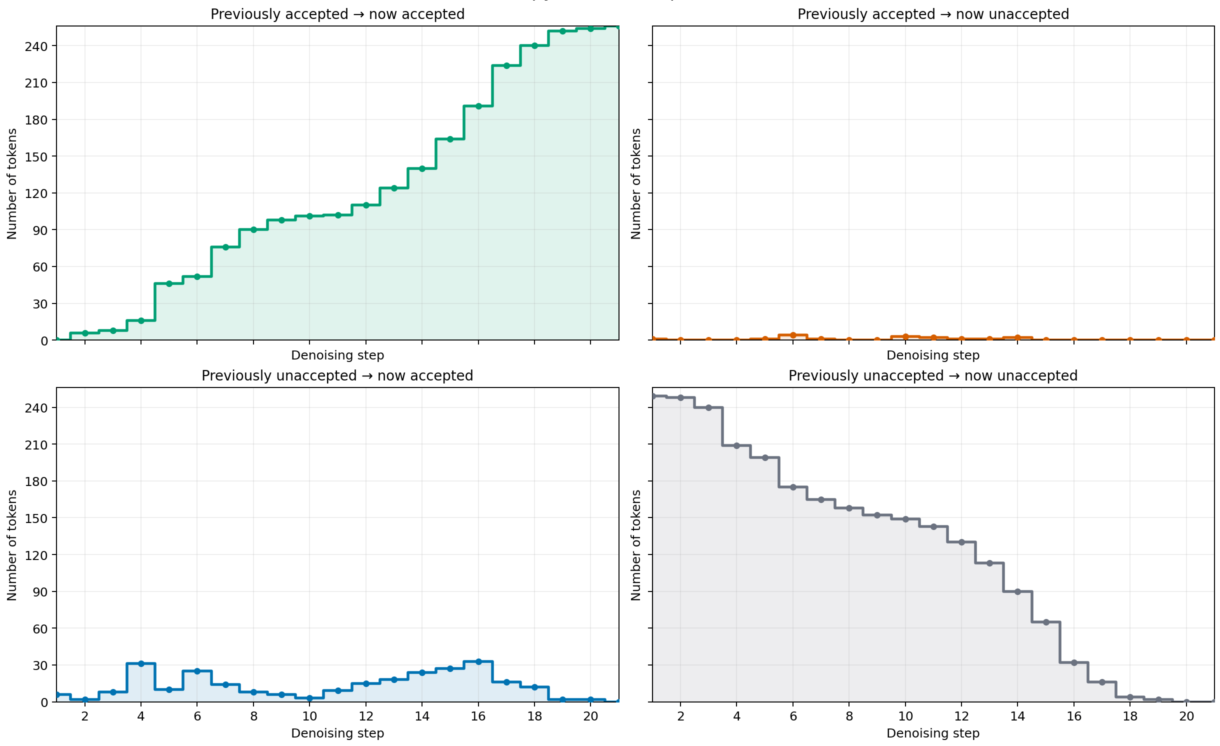
For 67 Prompt

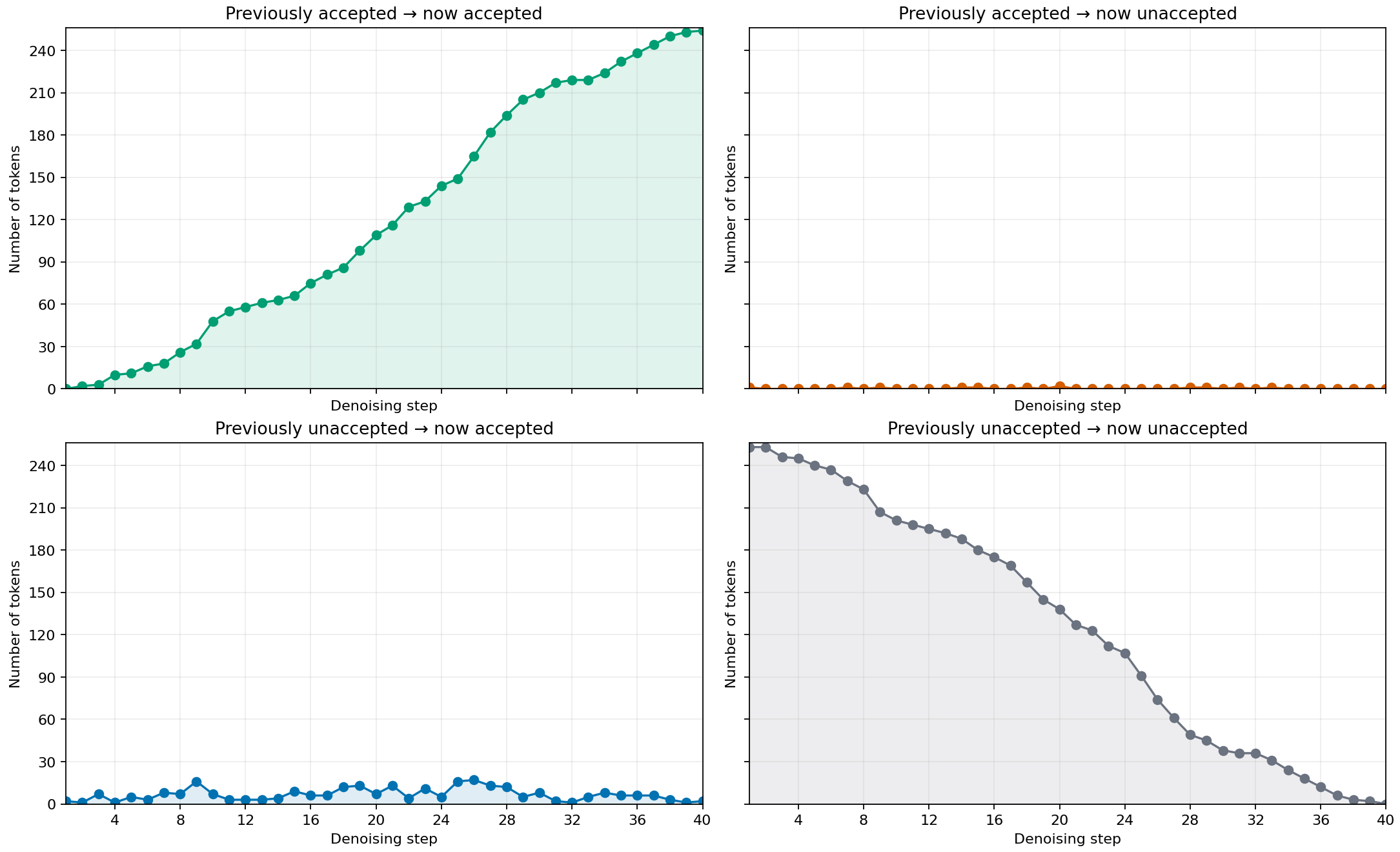
For Magic Square Prompt

Looking at the top right graph, almost no tokens are “re-masked” for both prompts. Google claims that one of the benefits of DiffusionGemma’s uniform state diffusion over traditional masked diffusion (e.g., LLaDA, Dream) is error correction via re-noising, but from our analysis, how often does that actually happen in practice?

• O’Donoghue, Brendan, and Sebastian Flennerhag. “DiffusionGemma: 4x faster text generation.” Google, 2026.

• Ballantyne, Ian, and Omar Sanseviero. “DiffusionGemma: The Developer Guide.” Google Developers Blog, 2026.

• Google AI for Developers. “DiffusionGemma model overview.” 2026.

• Google AI for Developers. “Diffusion in Text Generation Explained.” 2026.

• Google DeepMind. “DiffusionGemma 26B-A4B-IT model card.” Hugging Face, 2026.

• Google DeepMind. “DiffusionGemma reference sampler.” Gemma repository, 2026.

• vLLM Team and Google DeepMind Team. “DiffusionGemma: The First Diffusion LLM (dLLM) Natively Supported in vLLM.” vLLM Blog, 2026.

• Grootendorst, Maarten. “A Visual Guide to DiffusionGemma.” Exploring Language Models, 2026.

• Huang, Austin, Suraj Subramanian, Jonathan Sum, Khalid Almubarak, and Stella Biderman. “The Annotated Transformer.” Harvard NLP, 2022. Original version by Alexander M. Rush.

• Peng, Bowen, Jeffrey Quesnelle, Honglu Fan, and Enrico Shippole. “YaRN: Efficient Context Window Extension of Large Language Models.” arXiv:2309.00071, 2023.

• Su, Jianlin, et al. “RoFormer: Enhanced Transformer with Rotary Position Embedding.” arXiv:2104.09864, 2021.

• Kayyam, Ali, Anusha Madan Gopal, and M. Anthony Lewis. “Do Transformers Need Three Projections? Systematic Study of QKV Variants.” arXiv:2606.04032, 2026.

• Elhage, Nelson, et al. “A Mathematical Framework for Transformer Circuits.” Transformer Circuits Thread, 2021.

• Austin, Jacob, et al. “Sharded Matrices and How to Multiply Them.” How To Scale Your Model, 2025.

• Roos, Daan, et al. “Categorical Flow Maps.” arXiv:2602.12233, 2026.

• Nie, Shen, et al. “Large Language Diffusion Models.” arXiv:2502.09992, 2025.

• Ye, Jiacheng, et al. “Dream 7B: Diffusion Large Language Models.” arXiv:2508.15487, 2025.