
Suppose you have an initial value problem (an ordinary differential equation, ODE, with an initial condition):
\(\begin{cases} y’(t)=f(t,y(t)),\\ y(t_0)=y_0. \end{cases}\)
You want to approximate the solution at times
\(t_0,t_1,t_2,\dots\)
with a fixed step size h, i.e.
\(t_{n+1}=t_n+h.\)
The whole game is: how do we go from
\((t_n,y_n)\)
to
\((t_{n+1},y_{n+1})\)
without knowing the true curve solution?
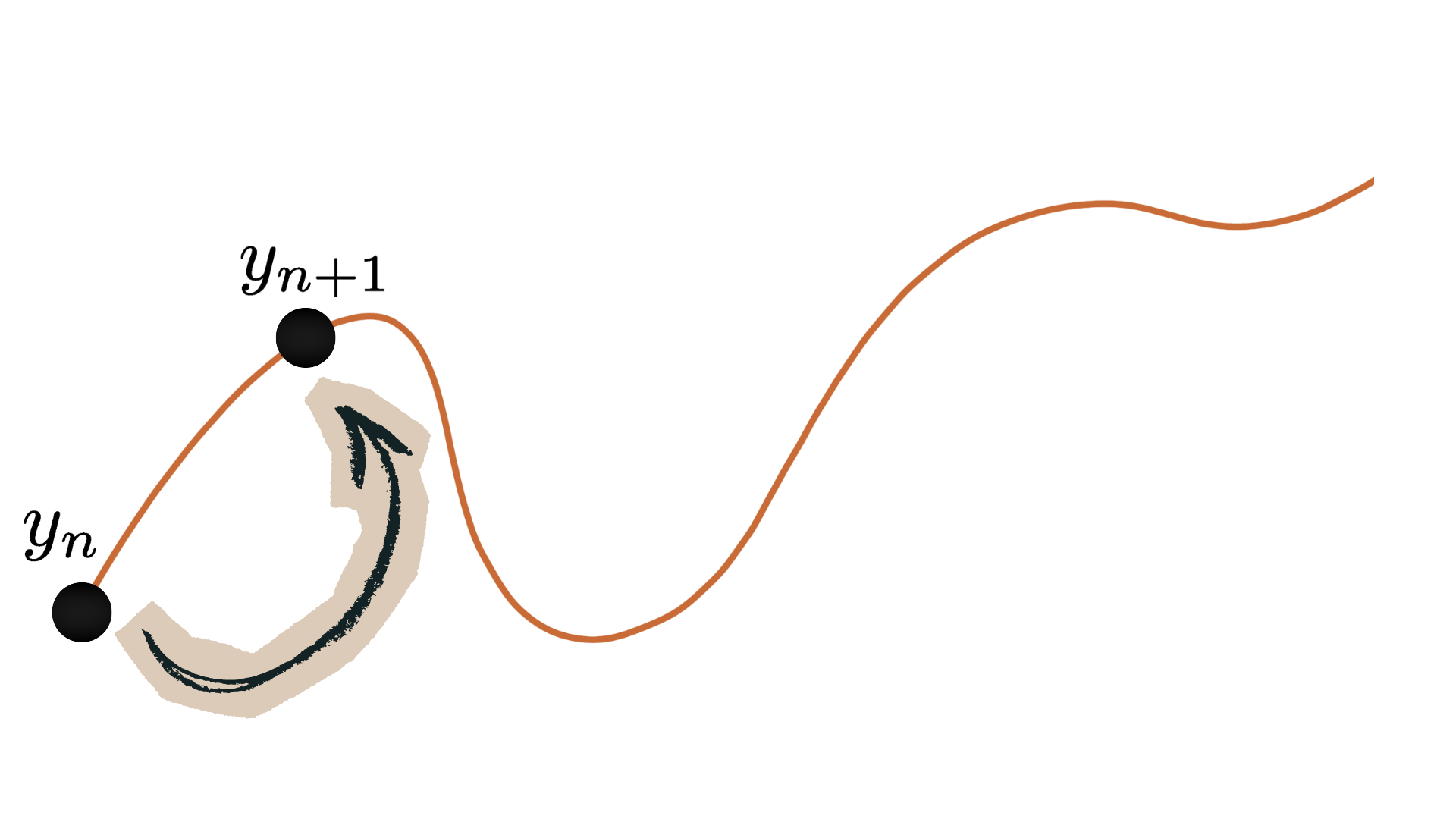
Euler’s method takes the derivative at the left endpoint and pretends it stays constant for one step:
\(y_{n+1}=y_n + h\,f(t_n,y_n).\)
This is fast, but it can be quite inaccurate: the slope usually changes during the interval.
So the natural upgrade is:
If the slope changes, don’t trust just one slope. Consider more.
A simple fix is to estimate the slope in the middle of the interval, where it’s often “more representative”:
compute the slope at the start:
\(k_1=f(t_n,y_n),\)
use it to predict a midpoint value:
\(y_n+\frac{h}{2}k_1\)
compute the midpoint slope:
\(k_2=f\!\left(t_n+\frac{h}{2},\,y_n+\frac{h}{2}k_1\right),\)
step using that slope:
\(y_{n+1}=y_n+h\,k_2.\)
This is another Runge–Kutta method: you take a few slopes and then combine them.
An explicit Runge–Kutta method with s “stages” looks like this:
\(\begin{aligned} k_1 &= f(t_n,y_n),\\ k_2 &= f\!\left(t_n+c_2h,\;y_n+h(a_{21}k_1)\right),\\ k_3 &= f\!\left(t_n+c_3h,\;y_n+h(a_{31}k_1+a_{32}k_2)\right),\\ &\ \vdots\\ k_s &= f\!\left(t_n+c_sh,\;y_n+h\sum_{j=1}^{s-1}a_{sj}k_j\right),\\ y_{n+1} &= y_n + h\sum_{i=1}^s b_i k_i. \end{aligned}\)
The coefficients
\((a_{ij},b_i,c_i),\,\,1\leq i,j\leq s,\)
tell you:
where you sample the slopes through the
\(c_i,\)
how each intermediate guess is built, the
\(a_{ij},\)
how to combine the slopes at the end, with the
\(b_i.\)
They’re often written in a compact “Butcher tableau”:

The classic 4th-order method (often just called “RK4”) uses four slopes:
\(\begin{aligned} k_1 &= f(t_n,y_n),\\ k_2 &= f\!\left(t_n+\tfrac{h}{2},\,y_n+\tfrac{h}{2}k_1\right),\\ k_3 &= f\!\left(t_n+\tfrac{h}{2},\,y_n+\tfrac{h}{2}k_2\right),\\ k_4 &= f(t_n+h,\,y_n+h\,k_3),\\ y_{n+1} &= y_n + \tfrac{h}{6}\left(k_1+2k_2+2k_3+k_4\right). \end{aligned}\)
If you stare at the final combination, it’s literally a weighted average of slopes, with extra weight on the “middle” ones.
Step size matters. Even a high-order method fails if h is too large for the dynamics you’re trying to resolve. (A fast-oscillating solution needs small steps.)
Stiff problems are special. For stiff equations, explicit RK methods can be forced to take absurdly small steps to remain stable. That’s where implicit RK methods (or other stiff solvers) enter.
We will discuss how to handle implicit Runge-Kutta methods and simulate ODEs with them in a separate post.
---
If you want more posts like this, consider subscribing to the newsletter and sharing the post:
No posts
Comments
Nothing yet. Say the first thing.
Sign in to join the conversation.