Inside the 1-Bit LLM: How Bonsai Fits a 27B Model on a Phone

In July 2026, PrismML shipped a 27-billion-parameter language model, built on Alibaba's Qwen3.6-27B, that runs in a browser tab on WebGPU and, separately, on a phone. The full-precision version of that model is 54 gigabytes. The one that fits in your pocket is under 4. This post is about how that gap gets closed, what the arithmetic behind it actually says, and where the honest line sits between what PrismML has disclosed about their method and what remains their own.

This is a free deep technical explainer through the whole conceptual pipeline: why phone-class hardware can't hold a normal LLM, the quantization math that makes 1-bit weights survive at all, the training pipeline that produces them, and an honest accounting of what PrismML has and hasn't told the public. The paid section below the fold is a hands-on payload: a worked plan for converting a small open model to ternary yourself on a single machine, with the code that makes the straight-through estimator concrete.

Start with the arithmetic nobody argues with. A model's parameter count and its file size are related by one multiplication:

size in bytes = parameters × (bits per weight / 8)

At FP16, the standard training and inference precision, that's 2 bytes per weight. A 27-billion-parameter model is therefore 27×10^9 × 2 bytes, which is 54 gigabytes.

The size number gets most of the attention, but it's not actually the bottleneck that matters for how the model feels to use. Generating text with an LLM one token at a time is a memory-bandwidth-bound operation, not a compute-bound one. Every single token requires streaming the model's entire weight set through memory once, and the amount of arithmetic done per byte fetched is small. That means time per token is approximately:

time per token ≈ model size in bytes / memory bandwidth in bytes per second

This is the number that actually decides whether a model feels usable. Shrinking the weights doesn't just make the file smaller, it directly cuts the time to generate each token, because the bottleneck is moving those bytes, not multiplying them. A phone's memory bandwidth is a small fraction of a workstation GPU's. The only way to make a 27B model livable there is to cut the bytes it has to move, not to find a faster way to multiply them.

Figure 1 lays this out directly. It contrasts the FLOPs required per token, which are cheap and not the constraint, against the bytes that have to be streamed from memory, which are the actual bottleneck. Cutting bytes per weight by roughly 14x, going from 16-bit down to about 1.1 bits, cuts decode latency by roughly the same factor. This is the entire mechanism. It's not that 1-bit arithmetic is faster per operation, though it is; it's that there's simply far less data to move.

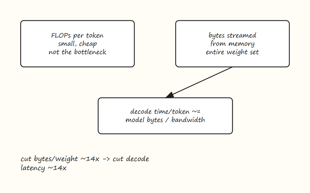
Figure 1: Memory Bandwidth Bound Decoding

So the actual engineering problem is: how far can you compress each weight before the model stops working, and what does it take to get there.

The compression method behind Bonsai is ternary quantization: every weight collapses to one of exactly three values, -1, 0, or +1, with one shared scaling factor per group of weights carrying the magnitude information that got thrown away.

The standard scheme, absmean quantization from the BitNet b1.58 line of work, computes a scale gamma as the mean absolute value of the weights in a tensor, then rounds each weight to the nearest of {-1, 0, +1} after dividing by that scale:

gamma = (1/n) × sum(|wi|) wtildei = clamp(round(wi / gamma), -1, 1)

Given a fixed rounding rule, the scale that minimizes squared reconstruction error is the least-squares projection of the weight tensor onto the chosen ternary pattern. Working that out gives the mean of |w| over the nonzero-assigned weights. Absmean over the whole tensor is a computationally cheap stand-in for that exact value, since it needs no threshold search and no second pass over the data, which matters because it gets recomputed constantly during training.

Now put a number on the damage. Model the trained weight distribution as Gaussian, w ~ N(0, sigma^2), the standard simplifying assumption for a weight tensor that's converged during training. Under that assumption:

gamma = E[|w|] = sigma × sqrt(2/pi) ≈ 0.798 × sigma

Rounding sends everything with |w| below gamma/2 ≈ 0.399 × sigma to zero. Integrating the Gaussian density over that band gives roughly 31 percent of all weights landing on zero. That's not a rounding footnote, that's a third of the tensor being deleted.

Figure 2 shows this geometrically: the weight distribution as a bell curve, with a dead zone in the middle that collapses to zero and two outer buckets that collapse to plus or minus one. The width of that dead zone, set by gamma/2, is what determines how much of the tensor survives as signal versus how much gets zeroed.

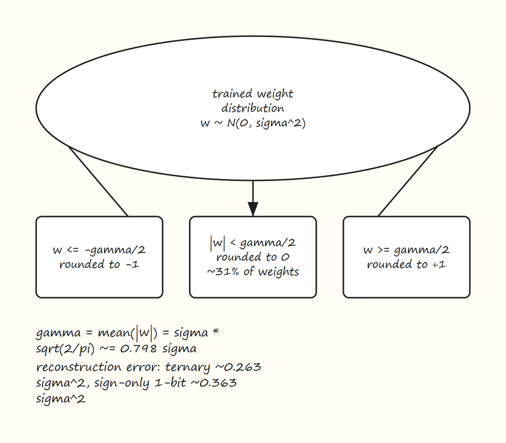
Figure 2: Absmean Ternary Rounding

Working out the expected squared reconstruction error E[(w - gamma × w_tilde)^2] under the same Gaussian assumption gives approximately:

ternary: 0.263 × sigma^2 1-bit sign-only (no zero state, {-1,+1} only): (1 - 2/pi) × sigma^2 ≈ 0.363 × sigma^2

Both of these are derived under the Gaussian assumption for this explanation; real trained-weight distributions are heavier-tailed, so treat the exact constants as illustrative rather than a spec. What they establish is the shape of the tradeoff. Ternary reconstruction error is roughly a quarter of the weight's own variance. That is not a small perturbation, the root-mean-square error is on the order of half the root-mean-square weight magnitude. A model cannot survive that kind of damage if you just round a trained network after the fact. It has to be trained to already sit in a place where this specific kind of rounding doesn't cost it much, which is the whole reason quantization-aware training exists and post-training rounding doesn't work at this bit depth. More on that below.

The gap between the two numbers, 0.263 versus 0.363, is also the quantitative story behind the retention figures PrismML has published: 94.6 percent for the ternary build, 89.5 percent for the 1-bit build, both measured against the FP16 baseline. The zero state costs about a third less reconstruction error than sign-only quantization, and that difference in error is what buys roughly five points of retained capability. The value of keeping zero isn't aesthetic, it shows up directly in this arithmetic.

A ternary symbol carries log2(3) ≈ 1.585 bits of information, not 1 and not 2. That's why you'll see the format referred to as "1.58-bit." But storing the symbols isn't the whole cost. You also need to store gamma, the scale factor, and how you amortize that scale across weights changes the total bits per weight substantially.

The general formula for any block-quantized format is:

bits per weight = payload bits + metadata bits / group size

Payload is what one weight symbol costs on its own. Metadata is the shared scale (and sometimes an offset) a block of weights split among themselves. Larger groups spread the metadata cost thinner but track the local weight distribution less precisely, since weight magnitude isn't actually uniform across a tensor, it varies by row and by region.

Apply that formula to the three formats relevant here. PrismML's 1-bit build uses a "g128" layout: one FP16 scale (16 bits) shared across a group of 128 weights, with a plain sign bit as the payload.

1 + 16/128 = 1 + 0.125 = 1.125 bits per weight

That 1.125 figure is publicly confirmed for the Bonsai 1-bit build, sourced from PrismML's own documentation. For ternary at the same g128 grouping, using the information-theoretic payload of log2(3):

1.585 + 16/128 = 1.71 bits per weight

llama.cpp's Q4K format, in contrast, is built from 256-weight superblocks split into 8 sub-blocks of 32 weights each. Every sub-block carries its own 6-bit scale and 6-bit min (Q4K is asymmetric, it stores an offset as well as a scale, since post-activation weight distributions aren't zero-centered), and the whole superblock carries two FP16 values that scale those 6-bit fields:

(256×4 + 8×(6+6) + 2×16) / 256 = (1024 + 96 + 32) / 256 = 1152/256 = 4.5 bits per weight

Table 1 puts these side by side against the file size that implies for a 27B model and the retention numbers where they're known. The jump from 4.5 down to 1.71 down to 1.125 bits per weight is not a linear cost curve, it's the reason the file sizes in the right-hand column shrink by roughly 3x and then again by 1.5x for a total drop of about 14x from FP16.

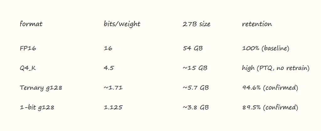
Table 1: Bits Per Weight and Retention

Figure 3 draws the same three formats as stacked bars, splitting each into its payload portion and its metadata-overhead portion, which makes the tradeoff visible: as the payload shrinks, the metadata term stops being a rounding error and starts being a meaningful fraction of the total.

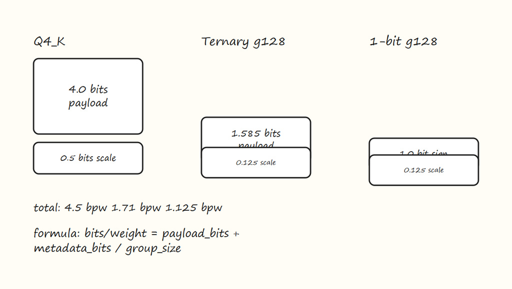
Figure 3: Bits Per Weight Breakdown

The group size choice is where the real design tension sits. Going from g128 to g32 would quadruple the metadata term, from 0.125 bits to 0.5 bits per weight. On a 1.125-bit format, that's a 44 percent size increase for the sake of finer-grained local scales, an expensive trade at this bit depth. On Q4_K's 4-bit payload, the equivalent overhead is a much smaller fraction of the total, which is exactly why formats built around 4-bit payloads can afford smaller groups and lower-bit formats can't. The lower you push the payload, the more disciplined you have to be about metadata, because there's nothing left to absorb it.

There are two ways to produce a quantized model. Post-training quantization, PTQ, trains a model normally and rounds the finished weights afterward. It's fast, needs no extra compute beyond the rounding pass itself, and it's what produces formats like Q4_K. It works because 16 quantization levels still track the real weight distribution closely enough that one-shot rounding doesn't do much damage.

Ternary and 1-bit don't have that luxury. As the error derivation above showed, rounding a trained FP16 model straight to three symbols throws away roughly a quarter of the weight's variance in one uncorrected shot. That damage is not recoverable by a better rounding rule; it's fundamentally too large a perturbation for the network to absorb after the fact. Below roughly 4 bits, PTQ stops being viable and quantization has to happen during training instead, quantization-aware training, QAT, so the model can compensate for the rounding as it happens rather than absorbing it as a fixed insult afterward.

The mechanical obstacle to doing this is that round() and clamp() are piecewise constant functions. Their derivative is zero almost everywhere and undefined at the jumps. A literal backward pass through the quantization step gives zero gradient, and zero gradient means no learning signal reaches the weight at all.

The straight-through estimator, STE, is the standard fix. The forward pass computes the real quantized value q(w) and the network runs on that. The backward pass, though, pretends the quantization step was the identity function inside the clipping range, so gradients pass through unchanged:

forward: y = q(w) · x the network only ever sees the rounded weight backward: treat q(w) as if it equaled w (straight-through estimator)

This is a deliberately incorrect gradient. It's justified as the gradient of a smoothed surrogate rather than the true quantization function, and empirically it works well enough to train through. Figure 4 draws both paths explicitly: the forward arrow running through the round/clamp box, and the backward arrow bypassing that box entirely as if it were transparent, with the discontinuity called out at the point where the two paths actually diverge.

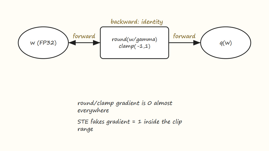
Figure 4: Straight Through Estimator

The practical consequence is worth sitting with. The full-precision weight that the optimizer updates is not really "the weight" in any functional sense, since the network never runs on it directly. It's an accumulator of evidence. The value that actually determines model behavior is the ternary symbol, and that symbol only changes when the latent FP32 value crosses a rounding boundary. Small gradients can accumulate quietly for many steps with no visible effect on the model's behavior, then flip a symbol discontinuously all at once. Training dynamics under STE look less like smooth gradient descent on the deployed function and more like a slow vote that occasionally flips a decision. That's a large part of why ternary conversions need long warm-up schedules and are sensitive to learning rate in ways a normal fine-tune isn't.

Weights aren't the only thing that gets quantized. Activations get quantized too, typically to int8, computed per token rather than per tensor, because LLM activations have severe outlier channels and a single global scale would let one outlier crush every other value to near zero.

Stack enough of these layers and a subtler problem shows up. Each ternary layer imposes a fresh multiplicative perturbation on its output's variance relative to what the FP16 model would have produced there. In a transformer, the residual stream carries every layer's output forward and adds the next layer's contribution on top, so these per-layer perturbations don't stay local, they compound with depth. This is the mechanism behind an empirical finding that shows up consistently in the quantization literature: the performance gap between an FP16 model and its ternary counterpart widens as models get bigger, not because bigger models are somehow more fragile in the abstract, but because there are more layers for the same per-layer variance drift to compound across.

SubLN is the fix used in the open BitNet Distillation architecture: an RMSNorm layer inserted immediately before each output projection inside a BitLinear block, re-pinning the activation scale at every layer before the next layer's ternary weights get a chance to compound the drift further. It's numerically a no-op at initialization, so it costs nothing to add, and its absence is a big part of why naive ternary conversions of large models tend to diverge where small ones don't.

Figure 5 traces the resulting forward pass through a single BitLinear block: input activations pass through SubLN first, then get quantized to int8, then meet the ternary-quantized weights at the matmul, producing the block's output. Every one of these steps is cheap on its own; the value of the whole arrangement is in keeping the compounding problem described above under control before it ever reaches the pipeline's warm-up stage, covered next.

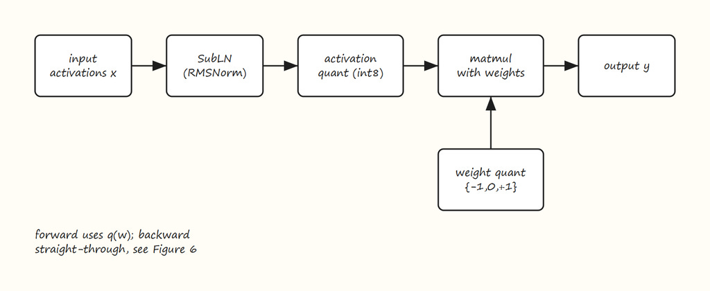
Figure 5: BitLinear Forward Pass

Everything from here through the end of the free section describes the open BitNet Distillation technique, published by Microsoft at arXiv:2510.13998 with code at github.com/microsoft/BitNet. I'm using it as a general explainer for how a pipeline of this shape works, not as a description of PrismML's actual undisclosed internals. Treat the two as separate claims: the mechanism below is publicly documented and reproducible; what PrismML specifically did to produce Bonsai is addressed honestly, and separately, in the next section.

The published pipeline runs in three stages, and the shape of the pipeline, not any single trick, is the actual contribution. Stage one is architecture surgery: every nn.Linear in the attention and MLP blocks gets replaced with a BitLinear module that applies the weight and activation quantization from earlier sections, and a SubLN gets inserted before each output projection as described above. This step is numerically a no-op at initialization, so it's essentially free.

Stage two is a continual pre-training warm-up: the now-ternary model trains on a general text corpus, with plain next-token cross-entropy, before it ever sees a teacher model or task-specific data. This is the step that's easiest to skip and the one that determines whether the whole approach works at scale. Because the FP16-to-ternary gap widens with model size, as covered above, a model that goes straight into distillation without this warm-up tends to diverge or plateau well below what the same pipeline achieves with it. The warm-up gives the ternary weights room to find a workable configuration before the constraint of matching a specific teacher's outputs gets layered on top.

Stage three is teacher distillation: a frozen FP16 copy of the original model runs alongside the ternary student, and the student trains against a combined loss of KL divergence between student and teacher logits (temperature around 2) plus MiniLM-style attention-relation distillation, which matches the student's query-key, key-key, and value-value relation matrices to the teacher's on the last layer. Logit distillation alone recovers most of the gap; the attention-relation term is what closes the remaining few points in the published results.

Figure 6 lays out all three stages left to right, with the frozen teacher shown feeding into stage three and the two loss terms labeled underneath it, and calls out stage two as the step most attempts at this conversion skip.

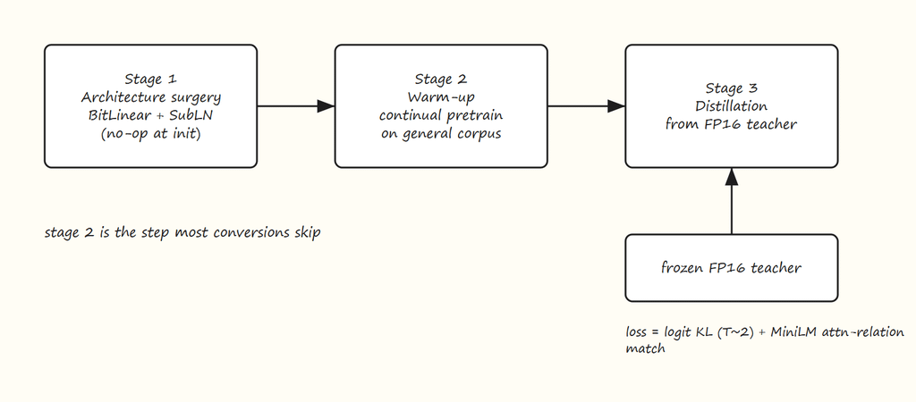
Figure 6: Three Stage BitDistill Pipeline

One thing worth separating clearly: WebGPU has nothing to do with why Bonsai is small. It's the browser's GPU API, and PrismML uses it so the model can run inside a page with no install step. The same GGUF weight file runs identically through llama.cpp on a CPU with zero GPU involvement, using the ternary-native tensor types TQ10 or TQ20 that upstream llama.cpp ships.

Figure 7 shows the same weight file feeding two entirely separate inference paths: a browser tab running WebGPU kernels for the zero-install demo experience, and a native llama.cpp process running CPU kernels for anyone who wants to run the model as an ordinary command-line tool. Both consume identical bytes. What differs is only which piece of software is doing the streaming and multiplying described back in Figure 5, not the compression that made the file small in the first place.

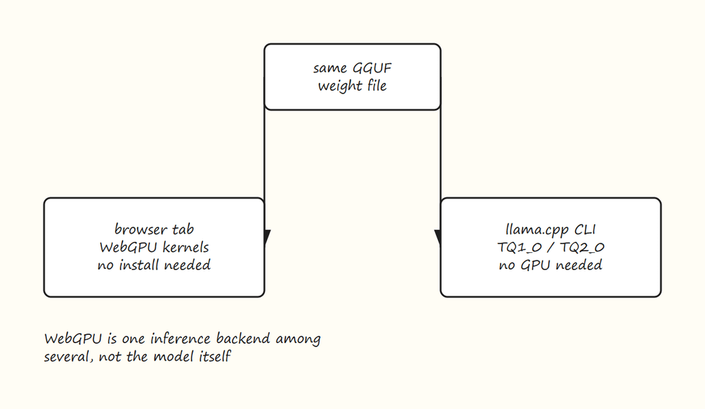
Figure 7: WebGPU Demo vs Native llama.cpp

This is worth being precise about, because it's easy to blur "how ternary conversion generally works" with "what this specific company disclosed," and those are different claims with different evidentiary weight.

Confirmed, and sourced directly from PrismML's own documentation at docs.prismml.com/models/bonsai-27b and from MarkTechPost's July 14, 2026 coverage: the base model is Qwen3.6-27B, the release is Apache 2.0 licensed, the weight format is g128 (one shared FP16 scale per 128 weights), the 1-bit build measures 1.125 effective bits per weight, and the reported retention numbers are 94.6 percent for the ternary build and 89.5 percent for the 1-bit build against the FP16 baseline.

Not disclosed: I went looking for training or quantization code directly on PrismML's GitHub organization. It has nine public repositories: a demo repo, an image-generation demo, forks of llama.cpp, mlx, and mlx-swift, an image-studio tool, an mflux fork, and two archived projects. Every one of them is inference or demo code. None of them is a training or quantization pipeline. A whitepaper file exists in the demo repository, but an attempt to extract its contents returned only raw, undecoded PDF binary data rather than readable text, so I can't respond to what's actually inside it and I'm not going to guess. If you want the specifics of their method, that PDF, read properly, is where to look, and I'd treat anything short of that as unconfirmed.

So the honest state of things is: the numbers above are real and public, the format is real and public, and the training recipe that produced them is not public. Everything in the pipeline section above is the general, independently documented BitNet Distillation technique, offered as the best available explanation of how a conversion of this shape works in principle, not as a claim about what's inside PrismML's proprietary run.

For paid subscribers, the rest of this post is a hands-on payload: a worked, step-by-step plan for converting a small open model to ternary yourself on a single machine, including the BitLinear code with the quantization and straight-through-estimator logic made concrete, the verification gates to run before committing to a full training run, and the evaluation and export steps to get from a trained checkpoint to a runnable GGUF file.

For paid subscribers — a hands-on deep dive continues below.

The Going Deeper section adds three things: (1) a concrete, runnable worked example with real code from the Claude Code and Hermes repositories; (2) a comparison of this pattern against MCP, A2A, and adjacent architectures, showing how and why this approach differs; and (3) project-driven Claude Code exercises — hands-on assignments you can build in realistic scenarios.

You can unlock this section — and every paid deep-dive across the whole Agentic AI and AI Security series — at 50% off a yearly subscription here: https://kenhuangus.substack.com/subscribe?coupon=302342d9.