
Earlier this month, I was honored to have been sponsored to attend the 16th International Conference on Climate Change in Washington DC, which was organized by the Heartland Institute and the CO2 Coalition.
Don’t worry, I wasn’t converted by the woke mind virus - the focus on this conference was on Climate Realism - not Climate Alarmism.
One of the keynote speakers was Nobel Laurete John Clauser.
John Francis Clauser (born December 1, 1942) is an American theoretical and experimental physicist who won the 2022 Nobel Prize in Physics, who shocked the Scientific Establishment in a high-profile talk at Quantum Korea 2023, where he declared there is no climate crisis, criticized climate models, called the IPCC “one of the worst sources of dangerous misinformation,” and argued that clouds (not CO₂) are the dominant factor in climate.
In his keynote speech, Dr. Clauser stated that throughout his career, he routinely spoke with God’s creation in his pioneering work in quantum information science.
This comment really resonated with me.
Another famous climate skeptic that has left a positive mark on my approach to discovering the nature of the forces at work in modern climate change was Dr. Tim Ball, former Senior Fellow with the Frontier Center for Public Policy - a role that I now am honored to fill within the Frontier Family.
In one of few conversations that I had with Dr. Tim Ball before his passing, he expressed his keen interest in my focus on atmospheric circulation patterns such as the Pacific easterlies (Trade Winds) or Walker Circulation dynamics. He argued that atmospheric circulation patterns undergo long term evolutions over time and that alarmists have largely overlooked this topic.
Dr. Tim Ball argued that the God Father of modern day climatology, H. H. Lamb who founded the Climatic Research Unit (CRU) at the University of East Anglia in 1972, placed a lot of weight on zonal and meridional wind speed records in his climate research.
As a southern Albertan rancher, I am keenly aware of the powerful moderating effect that changes in the relative strength of westerlies versus northerlies, have in determining whether a winter season will be bone crushingly cold or warm enough to wear tee-shirts outside in January.
We call these anomalously warm winter events Chinooks and they are characterized by strong westerlies, robust southerlies and elevated sunshine intensity (hours).
Arguably, it is my interest in Chinooks that inspired me to learn more about atmospheric circulation physics and indeed, I too view my studies on this topic as if I am attempting to communicate with God’s creation.
In this article, I will highlight evidence suggesting that Canada’s winter climate trajectory is defined by Pacific tropical climate trends, while Canada’s summer climate change is heavily modulated by the same forces as work in the North Atlantic.
1.0 Introduction
In this article, I will introduce you to a seasonal climate index that I have developed that foundationally, acknowledges that seasonal, interannual and decadal changes in near surface air temperature are all too often governed by or accompanied by changes in atmospheric circulation.
Before we dive into the methodology behind creating and interpreting these seasonal climate indexes, I will begin by building your general knowledge and appreciation for the fact that wind speed analysis is indeed pivotal in understanding the broader topic of climate science.
To start, I introduce Figure 1, which compares anomalies of the Pacific Trade Winds versus the Global average Westerlies. Note the deceleration and acceleration labels applied to both vertical axis and the fact that they are inverse to each other.
As I have discussed numerous times over the past year, a deceleration of the Pacific Trade Winds gives rise to what we know as an El Nino state in the Pacific tropics. This in turn is known to give rise to an acceleration in the global Westerlies through a mechanism called Bjerknes Feedback in atmospheric physics.
Bjerknes Feedback is simply the response of the subtropical to mid-latitude atmospheres to the release of stored thermal energy and rise in absorbed solar radiation in the Pacific tropics, as tropical clouds restructure during the collapse and reversal of Walker Circulation or Trade Winds during El Nino events.
This feedback gives to rise elevated rates of heat transport out of the Pacific tropics and into higher latitudes, where said heat is more readily able to escape through the top of the atmosphere along middle to polar latitudes.
Thus, when we see Westerlies anomalously rising as the Pacific Trade Winds anomalous decline, this signifies the simple fact that the entire planet is attempt to ventilate the pulse of excess energy released and generated in the Pacific tropics during El Nino events.
Conversely, the opposite is true during La Nina events and Pacific Trade Winds accelerate.
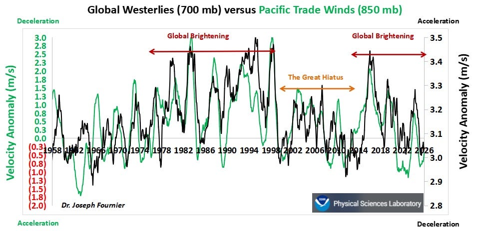
Figure 1. Pacific Trade Winds versus Global Westerlies.
It is the rise of the Westerlies during El Ninos, which force the development of Chinooks in southern Alberta along the eastern foothills of the Rocky Mountains. These air masses, originating in the west, effectively block winds from the north (Northerlies) from migrating to lower latitudes during the winter season.
I introduce Figure 2 to illustrate how the Earth’s rotation and the resulting Coriolis Force cause tropical air masses exiting the tropics, to be deflected towards the east as they move into middle to polar latitudes. Note how the purples arrows point towards the west along the equatorial latitude and how the green arrows point towards the east along the middle to polar latitudes.
Figure 2 also highlights classical nomenclature regarding the structure of counter rotating air masses called the Hadley, Ferrel and Polar Cells.
Note that during an El Nino event and the Trade Winds decelerate along the Intertropical Convergence Zone (ITCZ), the Hadley Cell expands towards higher latitudes and its rate of convection accelerates, pushing tropical air masses up into higher latitudes or into the Ferrel Cell.
It is in the Ferrel Cells where we see the strongest Westerly wind streams and thus the global average Westerlies is statistically biased towards the middle latitudes in either hemisphere.
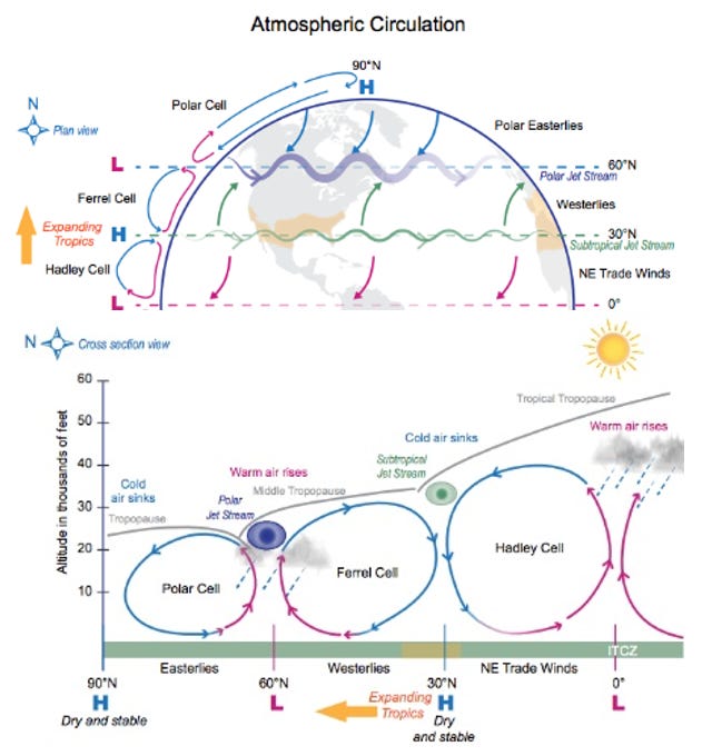
Figure 2. Classical model for global atmospheric circulation structures.
The next concept that I wish to emphasize is the idea that the Westerlies are at an annual maximum during the winter season when the surface temperature gradient between the oceans and land is at a maximum.
Figure 3 illustrates this characteristic by contrasting zonal (aka Westerly & Easterly) wind speeds by winter (Nov - Feb), spring (Mar - June) and summer (Jul - Oct) using 5-year averaging specific to the Northern Hemisphere. By using 5-year averaging, one is better able to visualize the long term or decadal trends in zonal winds by season.
Figure 3 clearly demonstrates that zonal winds are at a maximum during the Northern Hemisphere winter season and a minimum during the summer season.
As zonal winds are vector quantities, by convention Easterlies (i.e., Trade Winds) are asigned a negative sign and Westerlies are asigned a positive sign.
Thus, when Figure 1 shows the globally averaged Westerlies (Black) and we see a rapid spike towards positive values, this indicates that the Easterlies (Green) are decelerating.
The baseline used for the Easterlies (1950 - 1980) = -4.56 m/s and as the Easterly anomaly equation is:
Easterly anomaly = Monthly Average - Baseline = Monthly Average +4.56 m/s.
Therefore, a positively trending Easterly anomaly means the Monthly Average is collapsing to zero.
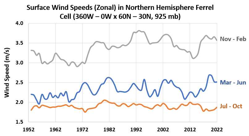
Figure 3. 5-year averaged zonal wind speeds for the Northern Hemisphere by season.
Building further the foundation of knowledge required to appreciate my climate index concept, I introduce the monthly average meridional wind speeds for the Northern Hemisphere.
Note that meridional means along longitudinal lines or north-to-south.
Southerlies and Northerlies are meridional winds.
Figure 4 shows that in the Northern Hemisphere, Southerlies (positive vector) statistically dominate from March to November and Northerlies (negative vector) from December to February.
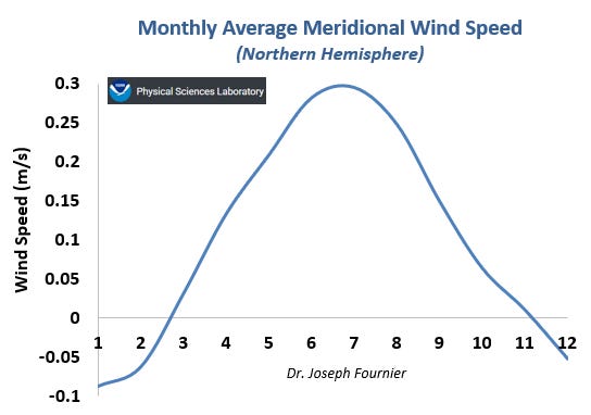
Figure 4. Monthly average meridional wind speeds for the Northern Hemisphere.
2.0 Methodology
We are now in a position to introduce three seasonal climate indexes, which in this analysis are defined by the following seasonal intervals:
Winter Climate Index - November to February.
Spring Climate Index - March to June.
Summer Climate Index - July to October.
Yes, I have redefined reality, by suggesting there are only three seasons. This is an arbitrary asignment - I could have used 3 month blocks, but I didn’t.
I have used NOAA’s National Centers for Environmental Prediction (NCEP) Reanalysis product to extract meridional and zonal wind speeds, together with lower tropospheric air temperature over Canada (140W - 50W x 70 N - 50N) at 700 mb, which is often referred to as the bottom of the free troposphere.
This monthly averaged data (e.g., meridional wind speed) was processed according to the following methodology:
Monthly averaged data was averaged into four month seasonal blocks (e.g., Nov - Feb) for each year over 1948 to 2025.
Each yearly seasonal block was asigned a baseline average over 1970 to 2000 and for which a standard deviation was quantified.
Each parameter (e.g., zonal wind speed) was then converted to an anomaly by subtracting the baseline from the yearly seasonal block value.
Each parameter (e.g., lower tropospheric air temperature) was then converted to an index by by dividing its anomaly by the baseline’s standard deviation.
Each parameter index was then converted into a 5-year rolling averaged time series to emphasize decadal (climatic) trends.
A seasonal climate index was then produced by averaging the seasonal block index for each of the three parameters into a single composite index.
When you think of the Winter Climate Index, think of wind chill.
By averaging each of the three parameter indexes, a statistical facsimile of atmospheric circulation is constructed.
By dividing each parameter anomaly by its standard deviation prior to averaging into a composite index, a positive bias is established for the parameter anomaly (e.g., lower tropospheric air temperature) with the smallest standard deviation.
3.0 Canadian Winter Climate Index
As a Southern Albertan sheep rancher, who lambs during the months of October to January, I am keenly biased to understand and prepare for anomalous winter season trends. During these months, I am extremely grateful for those weeks where prevailing winds are from the West and Southwest, while I dread those periods when when Westerlies decline and in their place the Northerlies bring in those monster Arctic airmasses with bone-breaking wind chills.
You know wind chills are deadly, when with even a balaklava face covering, your eyelids struggle to not freeze shut when facing into the northerly winds.
Figure 5 shows each of the three parameter indexes, together with the composite Winter Climate Index. The negative regions indicate that yearly seasonal block values are more negative or smaller in magnitude than the baseline value used in the construction of each of the parameter anomalies.
Note the prominent negative excursions shown in the Winter Climate Index, prior to 1976. During these intervals (e.g., 1966 to 1976), we find that the winter season block was defined by strong Northerlies, weak Westerlies and anomalously low air temperatures.
In fact, the most intense winter storm in Canadian history occurred in 1967 - a Southern Alberta claim to fame!
The intense decadal rise in Winter Climate Index from 1976 to the mid-1990s, was defined by a sudden growth in the strength of the Westerlies and Southerlies, together with an anomalous rise in lower tropospheric air temperatures.
Then suddenly, the mid-1990 peak Winter Climate Index gave way to a reversal of these positive trends and for the next 20 years, intensified negatively to a minimum around 2013, followed by a partial rebound into slightly positive territory between 2017 to 2025.
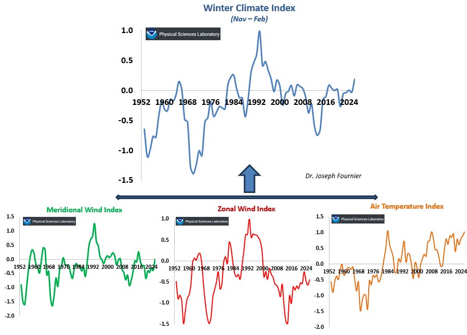
Figure 5. Canadian Winter Climate Index based on the average of the winter season meridional, zonal and lower tropospheric air temperature indexes.
The first steps that I took to determine if this Winter Climate Index was but a statistical construct, was to begin comparing to other classical atmospheric circulation indexes such as the Winter Arctic Oscillation (AO) and the Winter Pacific North American (PNA) Indexes (Figure 6).
The Winter AO is a large-scale atmospheric pressure pattern over the Northern Hemisphere. In its positive phase, low pressure over the Arctic strengthens the polar jet stream, keeping cold air north and bringing milder winters to mid-latitudes (North America/Europe). The negative phase weakens the jet, allowing cold Arctic outbreaks southward.
The Winter PNA Index describes a wave-like pressure pattern from the North Pacific to North America. Positive PNA features a deepened Aleutian Low, ridge over western North America, and trough in the east — typically warmer/drier in the west, cooler/wetter in the southeast U.S. in winter. A negative PNA pattern features a weakened Aleutian Low, a trough (lower pressure) over western North America, and a ridge (higher pressure) over the eastern United States, typically resulting in cooler and wetter conditions in the west and warmer, drier weather in the east during winter.
Both the AO and PNA strongly influence North American winter weather.
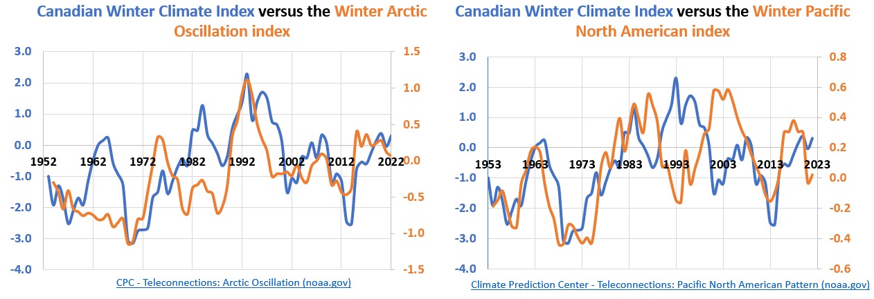
Figure 6. Comparisons of the Canadian Winter Climate Index to the Arctic Oscillation and Pacific North American Index.
While there are positively correlating intervals of time between both comparisons in Figure 6, I pressed on in my search as I was not entirely impressed with the temporal coincidence between the Winter Climate Index and the AO or PNA.
As I am obsessed with Pacific ocean - atmospheric processes, I turned to my old friend the Pacific Easterlies, which is of course the famous proxy for Walker Circulation within the World’s largest descrete climate regime, the Pacific Ocean.
The fact that we see this winter season correlation should likewise not be surprising, since we have already established that the Westerlies are the strongest during the winter season.
Figure 7 compares the 5-year averaged Pacific Easterlies versus the Canadian Winter Climate Index. I have added red stars to mark distinct periods where the positive correlation between the two time series breaks down.
These two intervals are 1960 to 1970 and again from 2020 to 2025.
Otherwise, Figure 7 shows a marked improvement in the temporal correlation between the Pacific Easterlies and the Canadian Winter Climate Index.
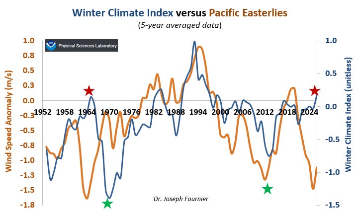
Figure 7. Canadian Winter Climate Index versus the Pacific Easterlies.
This stronger correlation with the Pacific Easterlies should not be a surprise, given what we have already established regarding the role of the Pacific Easterlies in dictating the the strength of the global Westerlies (zonal winds) and the blocking effect these winds have on winter season Northerlies.
The green stars coincide with two winter climate extremes from Canadian history.
The late 1960s green star coincides with the interval which saw the most intense winter storm in Canadian history (1967), while the 2013 green star coincides with the infamous Calgary regional food.
Both of these winter extreme were characterized by much the same atmospheric trends, which include deeply negative winter air temperatures, a late arrival of spring and highly persistent Northerlies over Westerlies.
Finally, the red star over 2025 is to aid the eye in visualizing the recent disconnect between the Winter Climate Index and the Pacific Easterlies. Canadians should be immensely grateful that the Winter Climate Index did not track the Pacific Easterlies into deeply negative territories during the recent three year La Nina (2020 - 2023).
Had this recent divergence not occurred, Canada would have experienced winter extremes not seen since the 1950s to 1970s.
We dodged a speeding bullet.
However, a downside to this divergence, has been the low snow packed reported across Canada over the past few years, resulting in reduced hydroelectric power generation and electricity imports from United States to cover the short fall.
This section concludes with an acknowledgement that Canada’s winter climate is strongly influenced by climatic changes occuring within the Pacific Ocean’s Walker Circulation zone.
4.0 Spring Climate Index
Figure 8 shows the Canadian Spring Climate Index, together with its parameter indexes. Note the differences in the magnitude of the vertical scale for the three parameters - they are relatively the same and thus contribute similarly to the scale and structure of the Spring Climate Index.
The deeply negative conditions of the 1950s to 1970s, is reminiscent of the Winter Climate Index. However, the Spring Climate Index underwent a near step change to more neutral conditions in the 1970s to 2000 and does not exhibit the mid-1990s peak positive conditions of the Winter Climate Index.
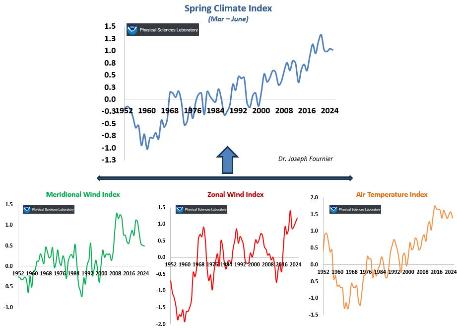
Figure 8. Canadian Spring Climate Index based on the average of the spring season meridional, zonal and lower tropospheric air temperature indexes.
Furthermore, around 2000 and continuing to 2025, the Spring Climate Index progressed into an increasing positive state, characterized by strengthening Southerlies since 2008, a step-change to more intense Westerlies around 2015 and a gradual warming of the lower troposphere from 2000 to 2017.
These changes in Canada’s Spring Climate are reminiscent of changes in sunshine intensity during the spring as reported by the Global Energy Balance Archive (GEBA) shown in Figure 9.
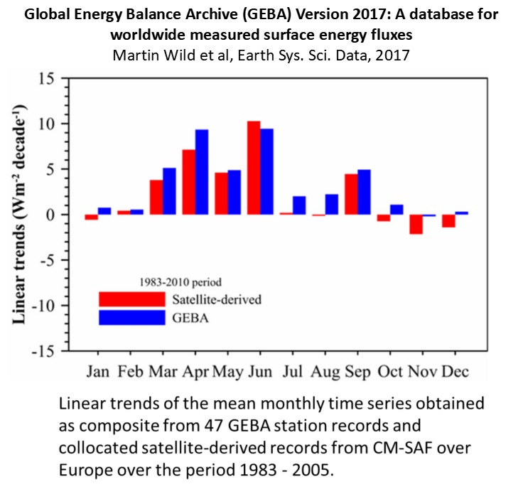
Figure 9. Change in sunshine intensity from 47 different European surface stations.
Likewise, the large positive growth in the Spring Climate Index is further reminscent of the progression of the Length of the Growing Season for Montana and Western United States from the 1950s to 2020, as shown in Figure 10. Since the 1950s, the North American interior has witnessed an expansion of the growing season by approximately three weeks.
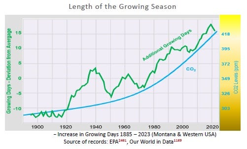
Figure 10. Increase in length of growing season over the 20th and 21st centuries in Montana and Western United States.
These collective changes are likewise analogous to the spring season’s snowcover extent, as reported by Ronan Connolly et al for the entire Northern Hemisphere (Figure 11). This adds credence to the idea that the growth in the Canadian Spring Index from the 11950s to 2025, was part of a hemispheric pattern of climate change, involving broad scale changes in atmospheric circulation, cloud cover, air temperatures and snowpack accumulation at higher elevations.
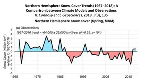
Figure 11. Northern Hemispheric spring season’s snowcover area anomaly.
This broad scale temporal association is extremely important to emphasize. All too often, alarmist voices point to changes in lower tropospheric air temperatures and snowcover as evidence of anthropogenic causation, while ignoring the context of atmospheric circulation and sunshine intensity changes occuring on the same time scales.
My opinion is that atmospheric circulation and sunshine intensity changes are causative, while changes in growing season length, snowcoverage and air temperature are their effects.
Like a domino chain - what mechanism drives these changes in atmospheric circulation and cloud coverage was alluded to in a recent article titled Beyond Milankovitch: Solar-Driven Atmospheric Dynamics in Neoglacial Evolution.
The prevailing mechanism within the current neoglacial phase of the Holocene Interglacial is climatic changes in the solar system.
Environment Canada should be ashamed, of how it has failed to collect sunshine data from its historical stations. I am confident that if it had been more responsible, it would have shown similar trends that European stations have over the same time interval.
5.0 Summer Climate Index
The next and final composite index is the Canadian Summer Climate Index, which Figure 12 shows to be characterized as rapidly falling from a peak in the 1940s, followed by a deep multi-decadal decline to the early 1960s, when a sudden natural tipping point to a multi-decadal positive phase emerged and that continues to 2025.
This sudden decrease in Summer Climate Index up the mid-1960s, is clearly seen in both the Zonal and lower tropospheric Air Temperature Index time series.
In this section, I have obstained from specifically calling Zonal winds, Westerlies, as there is a distinct possibility that Easterlies (negative vector) out of the North Atlantic climate zone likely rose following 2000. The intrusion of North Atlantic Easterlies over Central and Atlantic Canada since 2000, may be why we see the Zonal wind speed index moving towards zero in Figure 12 (i.e., averaging of a positive and a negative → 0).
The large sudden rise in Summer Climate Index around 1965, it largely due to a rapid increase in the zonal wind speeds from 1960 to 1970, followed by a gradual episodic rise in lower tropospheric air temperature starting around 1976.
On the otherhand, meridional winds show no clear trend from 1952 to 2000.
Come 2000, meridional winds transitioned to a prevailing Northerly direction, which is surprising given lower tropospheric air temperature made a significant positive advancement around the same time.
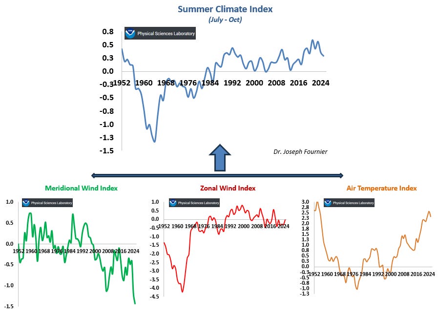
Figure 12. Canadian Summer Climate Index based on the average of the summwe season meridional, zonal and lower tropospheric air temperature indexes.
Given Central and Atlantic Canada border the North Atlantic, it is justified to see if the Canadian Summer Climate Index shows similar patterns of change with respect to the familiar Atlantic Multidecedal Oscillation (AMO) in sea surface temperatures.
The AMO is one of the most powerful natural climate regulators on Earth.
Figure 13 compares the Kaplan AMO time series to the Canadian Summer Climate Index, which shows that aside from the amplified negative correlation between both time series around 1960 to 1965, both time series show a consistent positive correlation from 1952 to 2025.
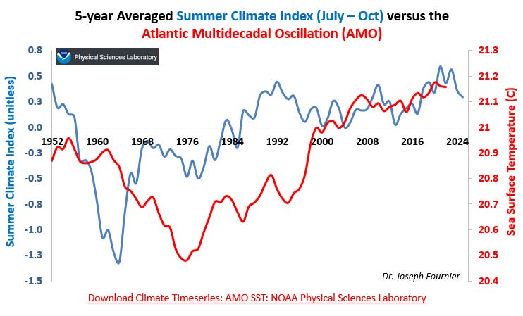
Figure 13. Comparing the Canadian Summer Climate Index with the Kaplan Atlantic Multi-decedal Oscillation (AMO) time series.
The idea that the Canadian Summer Climate Index is heavily influenced by the same forces shaping the multi-decedal changes in sea surface temperature in the North Atlantic should be no surprise. Figure 14 shows that it is during the Northern Hemisphere’s summer when the North Atlantic thermohaline (Atlantic Meridional Overturning Circulation or AMOC) reaches its annual maximum value.
This maximum annual value is of course a function of peak solar intensity and sunshine driven evaporation of surface water across the North Atlantic, which in turn gives rise to peak rates of deep water formation in the sub-polar North Atlantic Ocean.
Note that the AMO time shown in Figure 13 lacks the annual signal clearly visible in Figure 14, as it has been seasonally detrended using a 12-month rolling average.
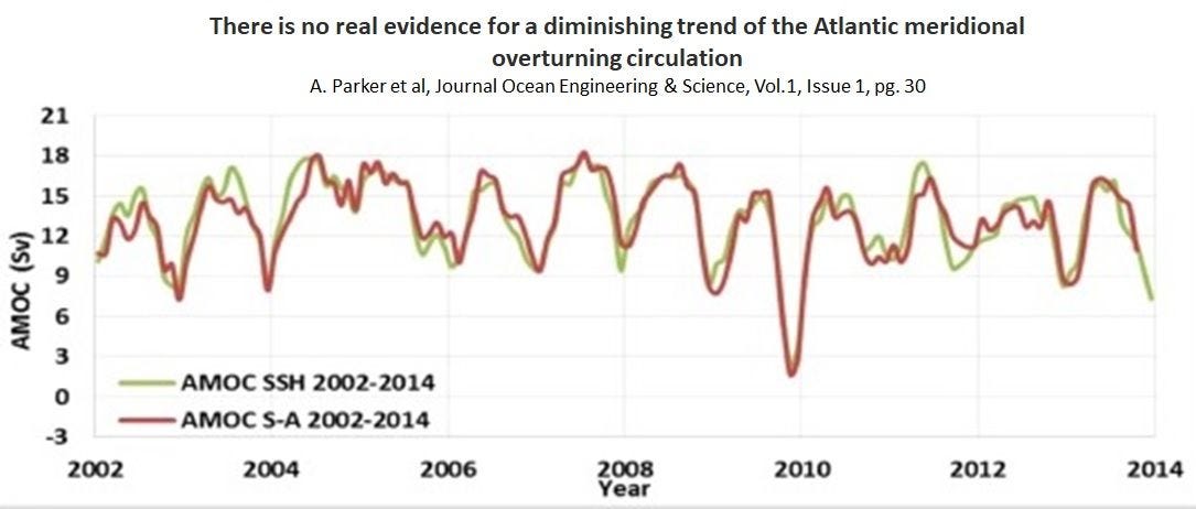
Figure 14. Early 21st century estimate of the Atlantic thermohaline circulation rate (AMOC).
Beyond the annual cycle and examining North Atlantic trends on a decadal basis, we see evidence of the same multi-decedal forces at work. Figure 15 shows recent literature suggesting that North Atlantic thermohaline heat transport (THC) sea surface temperatures and European sunshine duration (SD or hours) per year all show similar temporal trends to the Canadian Summer Climate Index (Figure 13).
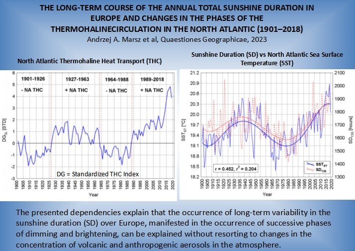
Oh, did I mention that these multi-decedal patterns in the North Atlantic are well known to be caused by changes in regional atmospheric circulation?
Indeed.
We call this pattern of atmospheric climate change the North Atlantic Oscillation (NAO) - for another article.
6.0 Conclusions
This analysis demonstrates that Canada’s seasonal climate variability is fundamentally governed by dynamic changes in atmospheric-oceanic circulation rather than trace greenhouse gases. By integrating zonal and meridional wind anomalies with lower tropospheric temperatures into composite seasonal indexes, a clearer picture emerges of natural climatic drivers at work since the end of WWII.
The Winter Climate Index reveals strong ties to Pacific Trade Wind (Walker Circulation) fluctuations, explaining historical extremes like the 1967 superstorm and the relatively mild recent winters despite La Niña conditions.
Spring Climate Index aligns with hemispheric trends in sunshine duration, snowcover retreat, and growing season extension—changes rooted in strengthened westerlies and southerlies, not solely CO₂.
Summer Climate Index track the Atlantic Multidecadal Oscillation and North Atlantic thermohaline strength, underscoring ocean-atmosphere coupling driven by solar intensity and evaporation cycles.
These indexes validate the insights of H.H. Lamb: clouds, circulation cells (Hadley, Ferrel, Polar), and Bjerknes Feedback dominate energy redistribution far more than model-projected CO₂ sensitivity.
Alarmist narratives overlook these mechanisms, misattributing circulation-driven warming and reduced snowpack to human causation while ignoring decadal wind cycles or natural tipping points.
As a southern Albertan rancher, I experience these realities directly through Chinooks, Arctic outbreaks, and lambing-season risks. Studying atmospheric physics feels like listening to God’s creation—humble observation over hubristic control.
Policymakers and agencies like Environment Canada should prioritize high-quality sunshine and wind data over simplistic temperature narratives. True climate realism demands we embrace natural variability, refine predictive tools around circulation physics, and reject fear-based agendas that ignore empirical evidence from Earth’s dynamic systems.
No posts
Comments
Nothing yet. Say the first thing.
Sign in to join the conversation.