Understanding Transformers (Part 4): Attention is just a few matrices

This week, I am picking up where we left off: moving beyond word embeddings and positional encodings, and stepping directly into the core magic of the Transformer: self-attention.

But before we can even talk about multi-heads or decoder stacks, we need to answer one crucial question:

➡️ How does a Transformer actually mix information across an entire sentence — all at once?

In this post, we will break down the full flow of the Scaled Dot-Product Attention mechanism:

• How words are compared through queries and keys,

• Why scaling and softmax are critical steps,

• And how new, context-rich representations are built by blending Value vectors.

All of this comes down to just a few simple matrix multiplications.

Let’s decode the full life cycle of a word inside self-attention.

• ✅ Understanding Transformers (Part 1): Why RNNs are nearly impossible to train

• ✅ Understanding Transformers (Part 2): How LSTMs fixed Recurrent Networks (mostly)

• ✅ Understanding Transformers (Part 3): Positional encodings and word embeddings

• 📌 Understanding Transformers (Part 4): Attention is just a few matrices (this blog post!)

• Understanding Transformers (Part 5): The final quiet layers doing some heavy lifting (coming soon!)

1. Positional encoding recap from part 3.

2. The dreaded diagrams (again)

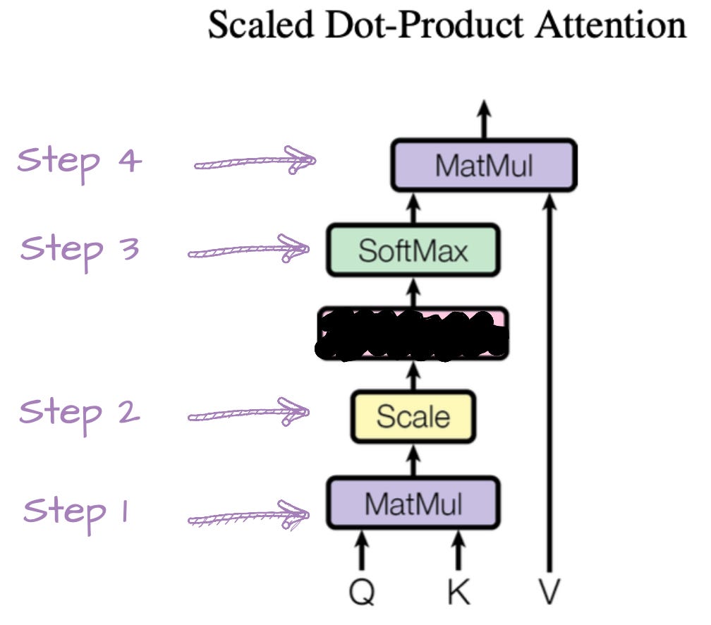
3. The 4 steps of the Attention mechanism

4. A short recap of self-attention

5. Scaling attention through multiple heads

Last time, we looked at the first stop every token makes when entering a Transformer: the combination of word embeddings and positional encodings.

On their own, word embeddings give us a sense of what a word means. "Cake" lives closer to "pie" than it does to "keyboard". But embeddings alone are location-blind: the model knows what is in the sentence, but not where.

So we added positional encodings that help the model keep track of order. With this, a Transformer knows that "The dog sat on the couch" is not the same as "The couch sat on the dog" (unless you are in the weird part of the internet).

By the end of this step every token in a sentence is now represented as a single vector (which combines what the word means with where it sits in the sentence).

Let’s take a simple sentence:

"I ate the cake and it was delicious."

• The model knows that “cake” is food (word embedding).

• It also knows that “it” appears later (positional encoding).

• But how does it know that "it" refers to the cake — and not to "I"? How can it link the word “delicious” back to cake?

This is the real limitation of positional encoding. It gives us structure, but not relationship. This is where attention comes in.

Whatever comes out of this embedding + position phase becomes the input to the attention mechanism. The next stage is about deciding:

➡ Which words should each token actually pay attention to?

Time to meet (again) the diagram that started it all...

I know, I have a habit of welcoming you with the scary technical diagrams pulled straight from academic papers. But as always, I promise we will break them down step by step, and by the end, they will feel a lot less intimidating. So, bear with me (again)

As we saw in Part 3, Transformers are built from multiple moving parts. This architecture comes from the original 2017 paper, Attention is all you need. In the diagram below, you can see that we will focus only on the blue-highlighted boxes — the ones labelled Multi-Head Attention.

That is where self-attention lives.

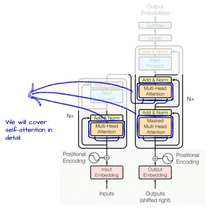
Luckily for us, the paper includes a zoom-in diagram of what is going on inside those boxes. That is what we will mostly focus on today: the Scaled Dot-Product Attention diagram (the one on the left).

You will also see an extra pink box labelled “Mask (opt.)” — this is only used during training for certain cases (like in the decoder). Since this post is focused on the mechanics of vanilla self-attention, we are going to skip it.

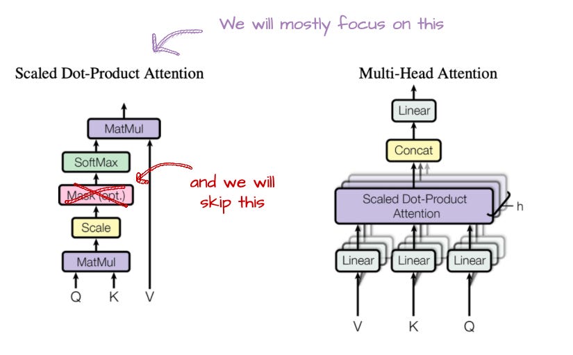
Now, let me guess — this still makes absolutely no sense.

You are probably asking:

• What are these Q, K, V?

• What are the 4 steps being followed in the Scaled Dot-Product Attention diagram?

• Why are Q and K “together”, but V follows a different path?

Well, you are in the right place to answer these and more questions. Lets cover all of this in the next phase!

If you take a look at the Scaled Dot-Product Attention diagram, you will see three mysterious vectors as inputs: Q, K, and V.

Before we dive into the maths, let’s take a detour into something you probably use every day: a recommendation system like Netflix (which I assume you have used at some point in your life).

Let’s say you are opening Netflix and searching for “science fiction”. What happens behind the scenes?

1. You make a query. You are saying, “Show me stuff that matches science fiction”.
   → This is your Q: the Query.

2. The system compares your query against a catalogue of options. Each film or show has some tags or features: action, drama, thriller, sci-fi, rom-com...
   → These are the K: the Keys — metadata or labels for each item.

3. Once the system finds the matches, it needs to know what to recommend.
   Not just the title, but also the thumbnail, the rating, or maybe a trailer preview.
   → These are the V: the Values — the actual information you receive.

So:

• Q = what you are searching for

• K = how each item is labelled

• V = what you get back if it is a match

The system compares your query (Q) to the keys (K), figures out what is most relevant, and then returns the values (V) for those relevant items.

Now let’s bring it back to Transformers.

In Transformers, we are not recommending TV shows. We are working with words in a sentence. But the mechanism is surprisingly similar. Let’s say we are looking at the word "it" in the sentence:

"I ate the cake and it was delicious."

• Q = a numerical representation of the word "it" (our query — what “it” is trying to understand)

• K = a set of keys for every word in the sentence (like "cake", "ate", "and", etc.)

• V = the values tied to those words — the actual information we might want to pull from them

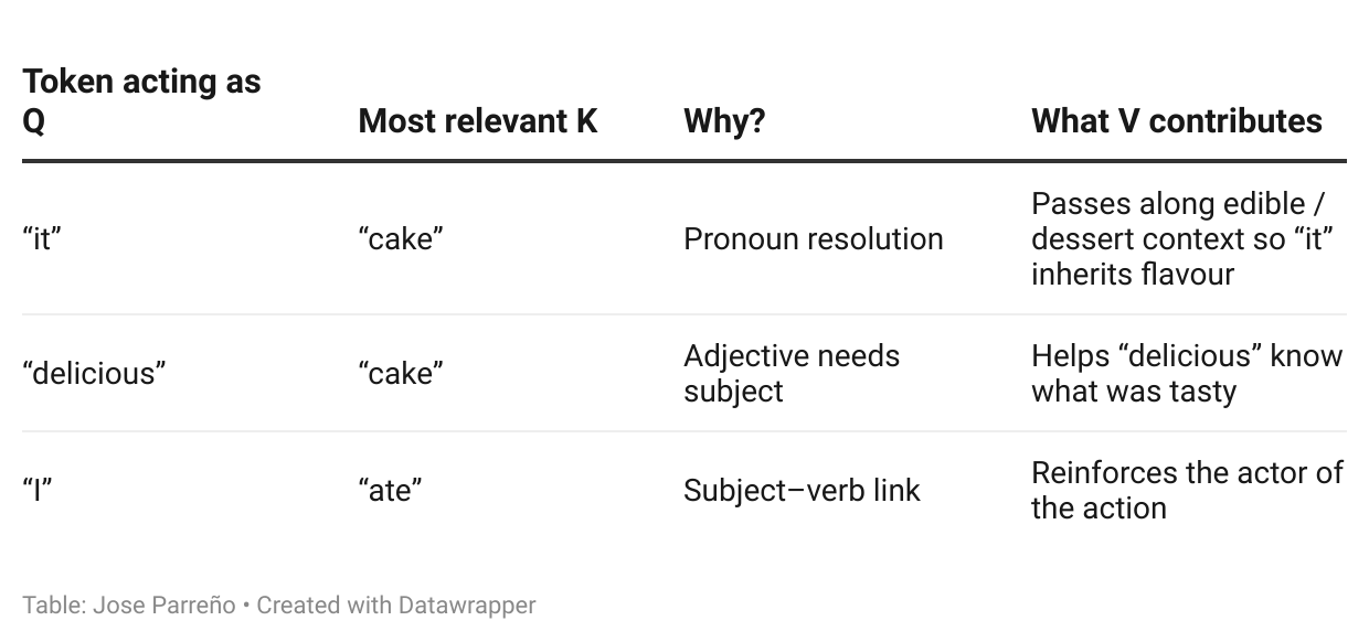
The goal is for “it” to attend to “cake”, not “and” or “I”. Just like Netflix aims to serve up Star Wars, not Love Island, when you search for sci-fi.

In the next section, we will go from intuition to mechanics:

• What do these Q, K, and V vectors look like mathematically?

• How are they built inside the Transformer?

But hopefully by now, you have a mental model:

Q is the seeker
K is what it is comparing against (catalogue of all tokens)
V is what it will get in return — weighted by how strong the match was.

I always wonder why do we have to be so mysterious in technical papers. Why call it MatMul instead of simply, matrix multiplication? Anyway, that is my little vent off for the day.

Let’s focus on the first step of the Scaled Dot-product attention diagram.

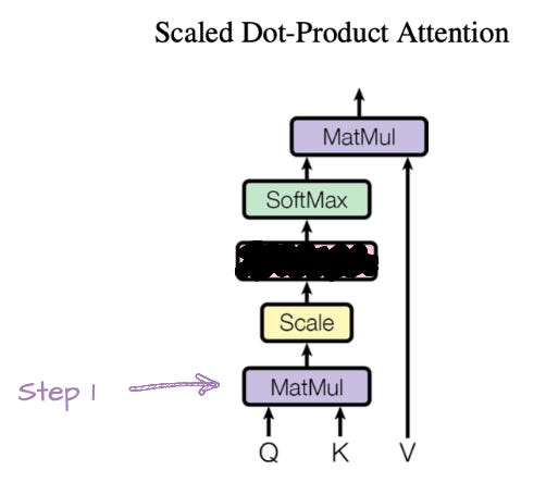
Let’s continue with our working example:

"I ate the cake and it was delicious."

After passing through the embedding and positional encoding layers, each word becomes a numerical vector that captures both meaning and position.
For simplicity, let us assume these are 4-dimensional vectors (see the red boxes below).

Each word embedding gets “pushed” through the matrices Wq and Wk to become a new vector.

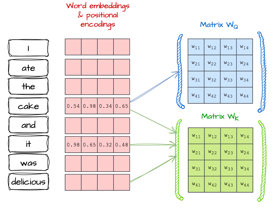
It simply means applying a linear transformation: We multiply the word’s embedding vector by the matrix, using standard matrix multiplication rules.

In plain terms:

• We take the embedding vector

• We do a dot product with each column of the matrix

• This gives us a new vector

To see what the simple dot product maths looks like, check the diagram below.

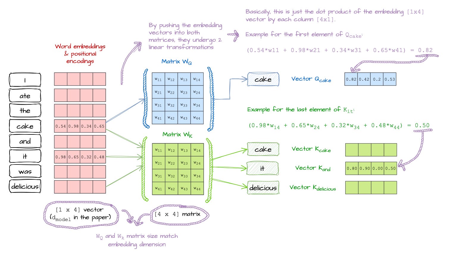
Let’s break this down bit by bit, going left to right:

• First focus on the dimensions of the vectors and the matrix. Notice that:

  • Each word is a [1 × 4] vector.

  • Each matrix is [4 × 4]

  • The 4 in the word vector (its number of elements) must match the 4 in the matrix (number of rows) for the multiplication to work.

• Now, lets focus on the vector Qcake.

  • It is calculated by multiplying the cake embedding vector by Wq.

  • Each value in Qcake is the dot product between the cake embedding and a column of Wq.

  • In the example above, we show how the 1st element of the Qcake vector is computed.

• Similarly, for Kit vector:

  • We take the embedding vector for "it",

  • Multiply it by Wk,

  • And compute each element the same way.

  • In the diagram, we show the last element of the Kit vector as an example.

Once we have projected the embeddings through the weights of the Q and K matrices, we are ready to compute the MatMul of Q and Kᵀ.

The diagram below shows an example:

• How the Qcake vector interacts with the Kit vector.

• How Qcake would similarly be compared to every other word in the sentence.

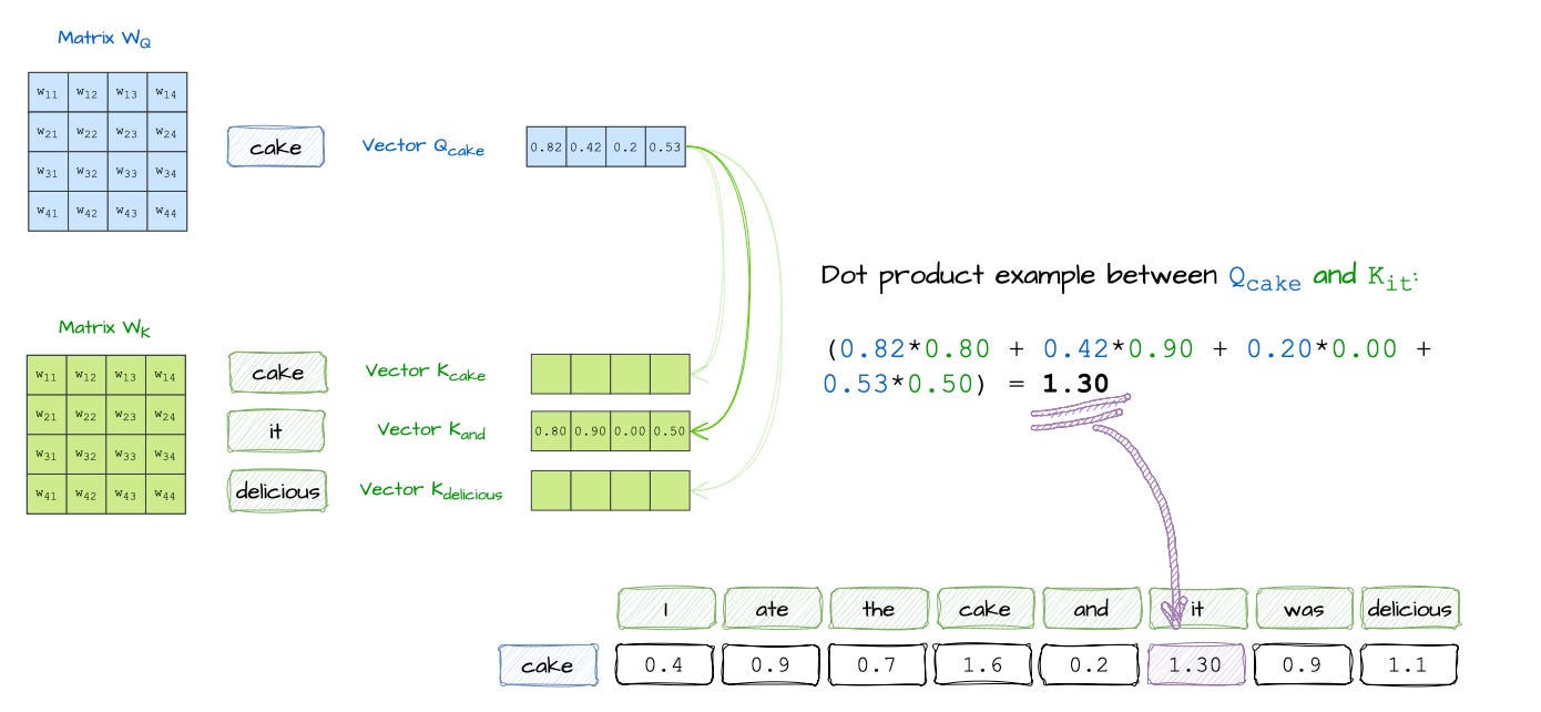
What happens here?

Each word acts as a query (Q) and is compared to all words as keys (K). The output is:

• 1 row per query word (in this case, "cake").

• 1 column per key word (every word in the sentence).

• Each cell in this row captures how similar the query is to that key.

For example:

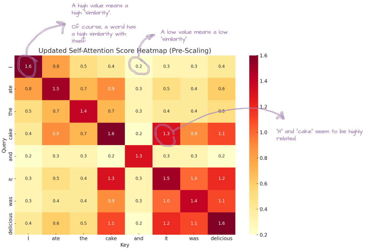
• “Cake” and “it” score 1.3 — strong similarity.

• “Cake” and “I” score 0.4 — much weaker.

In the full Transformer, we repeat this operation for every word, comparing each query to all keys. The result is a full similarity matrix — showing how much attention each word gives to every other word. Here is what a similarity matrix might look like:

Fantastic! So, now we have covered what the output of this first step looks like. Let’s move now to the “Scale” step.

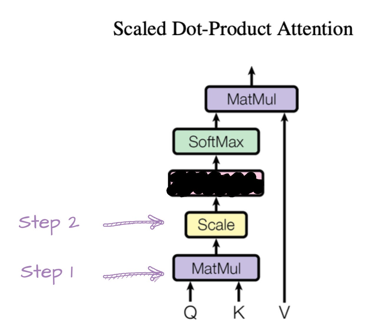
We now have a full matrix of similarity scores, where each word (as a query) has compared itself to every other word (as a key). But there is 1 problem.

Some of these numbers are already quite large (for example, 1.6 when a word compares to itself), even though we are only working with small 4-dimensional vectors. Imagine what would happen if we were working with embedding vectors of 512 or even 1024 dimensions — which is common in real Transformers.

Those dot product scores could grow very large, very quickly.

Because in the next step, we are going to apply a Softmax. And softmax is extremely sensitive to the scale of its inputs.

• If the numbers are too large, softmax becomes very "peaky" — it pushes almost all the probability mass onto one word, and nearly zero elsewhere.

• This makes the model brittle — small changes in input can cause huge changes in output.

• It also makes learning harder because the gradients become tiny and unstable.

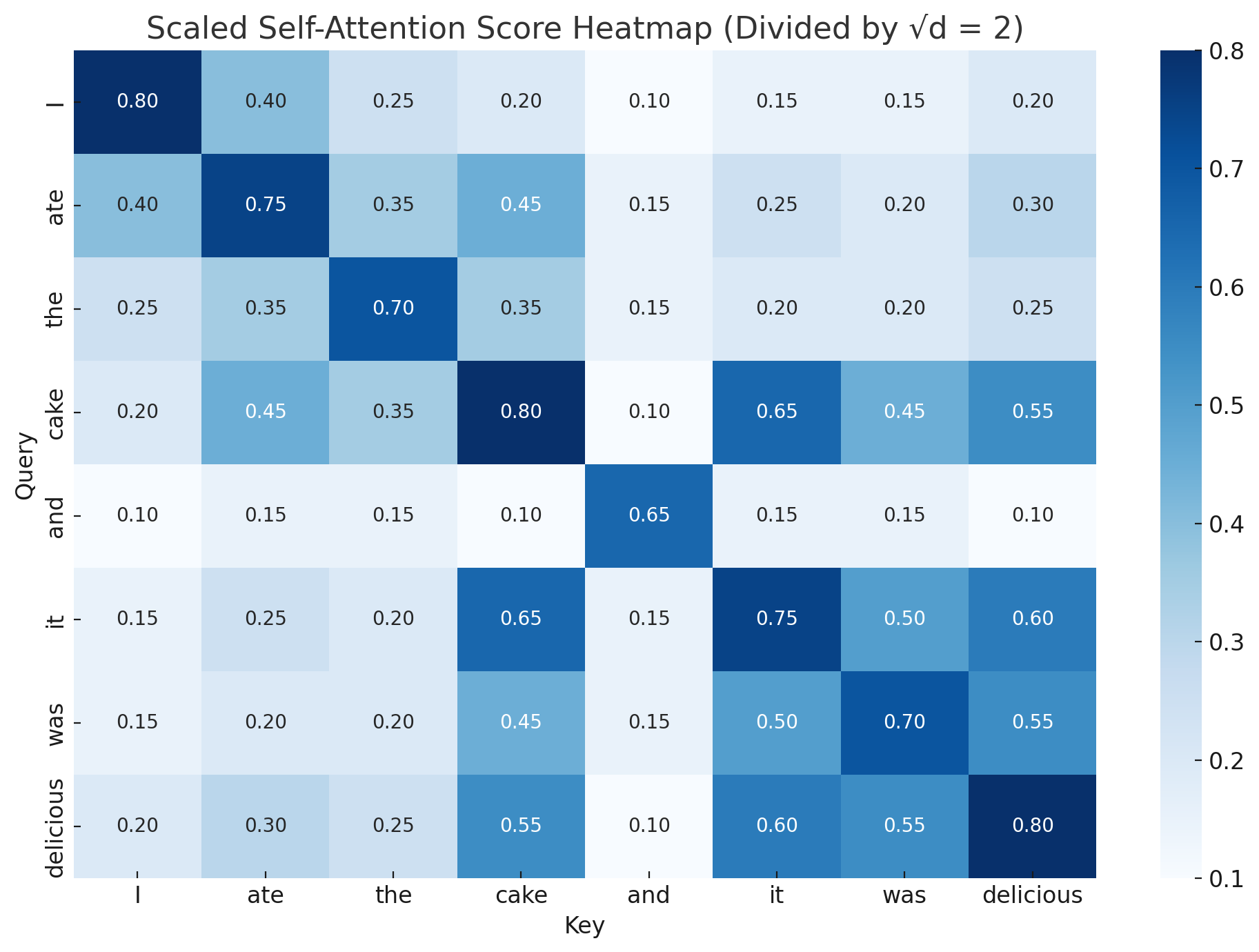
Instead of feeding raw dot products into softmax, we first divide each score by a number. Specifically, the square root of the vector size (√d).

In our toy example, since each vector has 4 dimensions:

Thus, every score would be divided by 2 before moving on to softmax. This simple trick controls the magnitude of the scores, keeping softmax outputs stable and making it easier for the model to learn.

Think of this like preparing water for coffee:

• If the water is too hot (raw dot products), the coffee burns and tastes awful (softmax explodes).

• If you scale it to the right temperature first, you brew the perfect cup (softmax behaves nicely).

With the scores now scaled, the next step is to turn them into probabilities using Softmax.

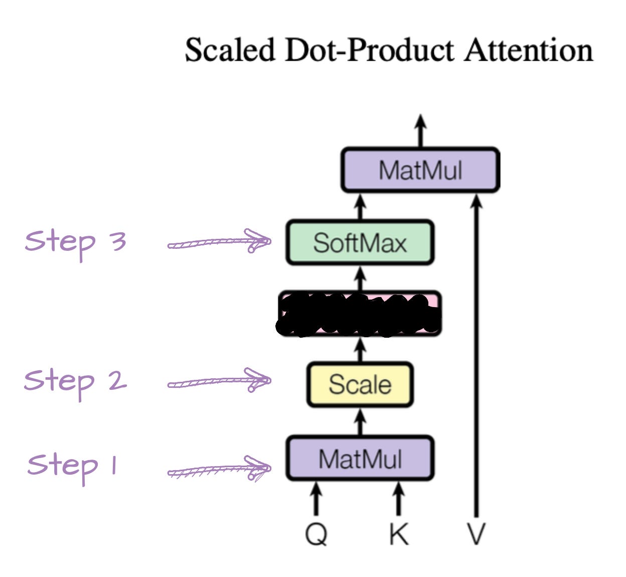
Now that we have scaled the scores, there is one more crucial step: turning these raw numbers into probabilities.

The scaled scores tell us how similar each query is to every key — but they are still raw numbers.
We want to turn them into something interpretable:

• Positive numbers between 0 and 1

• Where each row sums exactly to 1

• So that we can treat them like probability distributions over the words

Without Softmax, the model would not know how much relative "importance" to assign to each word.

Softmax is a simple mathematical function:

Where:

• zi is the i-th score in the row

• e^zi​ is the exponential of the score (making all outputs positive)

• The denominator sums over all scores in the row to normalise (let me stress out again, that softmax is applied row-wise)

• Another added bonus of softmax is that, it helps bring some non-linearity to the similarity between Q and K. In other words, it can learn some slightly more complex interactions between words that a simple dot-product (linear transformation) might miss.

Check how the attention heatmap looks like now.

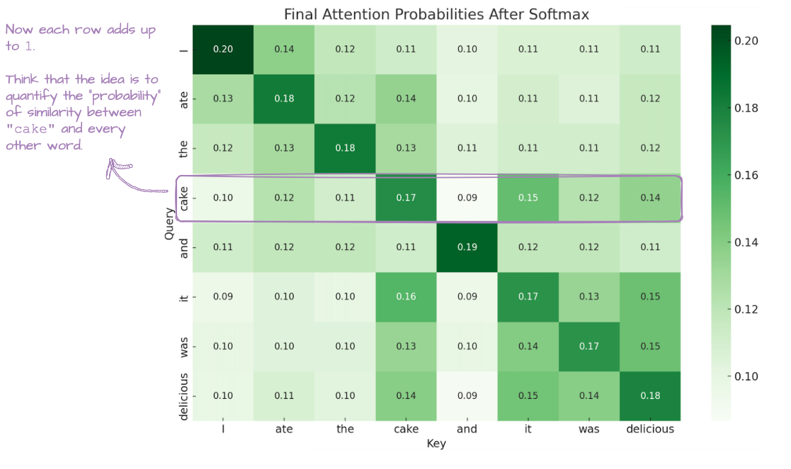
Now that we have turned our attention scores into clean probabilities, it is time to use them for something useful.

Specifically: we are going to combine information from the other words — using the V vectors.

Now that we have our attention probabilities, it is time to use them. We do this by performing one last matrix multiplication: Softmax matrix × Value matrix (V).

It looks similar to the Q × Kᵀ multiplication we did earlier, but here, we are not computing similarities. We are gathering information, using the attention probabilities as weights.

We already covered the matrix multiplication earlier on with Q × Kᵀ. The mechanics here are the same. For example:

• The self-attention softmax matrix has dimensions [n × n]: one row per query, one column per key.

• The V matrix has dimensions [n × dv]: one row per key, each a dv-dimensional vector.

• If we multiply these matrices, we get a resulting one with dimensions [n x dv]. In other words, 1 vector per word.

The operation is super easy:

• For each word (row) in the softmax matrix, take each element of the row and multiply it by the first element in the V vector.

• Add them up to get the first element of the new word vector.

• Repeat for all columns to built this [n x dv] vector.

In the diagram below you can see how we calculate the value of the first element of the Vcake vector.

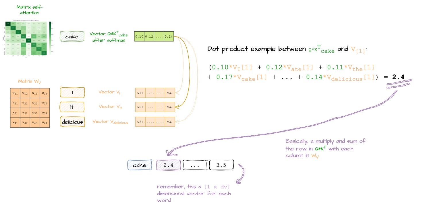
⚠️ Very important: The resulting vectors are not probabilities. In fact, you can already see it in the diagram → the number "2.4" we computed is completely fine.
(And outputs can be negative too.). The probabilities coming from the softmax just control how much V contributes to each word.

🎬 Think of it like browsing Netflix:

• The attention probabilities are like how much interest you have in movies. Maybe 25% Star Wars, 20% Interstellar, 10% Chef, and so on.

• But the actual movies (the V vectors) have their own characteristics:

  • Star Wars → [adventure 8, humour 2, 121 min]

  • Interstellar → [adventure 7, humour 1, 169 min]

  • Chef → [adventure 3, humour 6, 114 min]

• When you blend these 2 matrices with a matrix multiplication, you get your “personal movie” mood:

  Personal mood = 0.25*(8,2,121) + 0.20*(7,1,169) + 0.10*(3,6,114) + …

  = (6.9 adventure, 2.4 humour, 137 min)

📝 If we bring this back to our toy example:

• From the attention probabilities, we know that “cake” is related to “it” but not to “and”.

• The V vectors now represent something like an info-card. For example, each vector in V can represent dimensions such as [plural, 3rd person, noun, verb, entity, etc]

  • I → [plural = 0, 3rd person = 0, noun = 0, verb = 0, entity = human…]

  • ate → [plural = 0, 3rd person = 0, noun = 0, verb = 1, entity = action…]

  • cake → [plural = 0, 3rd person = 0, noun = 1, verb = 0, entity = dessert…]

When we multiply attention weights by these hidden features,
we blend meanings together.

The output vector for "cake" might now carry traces of:

• Being an entity (dessert),

• Being eaten (verb),

• Being referenced by "it" (pronoun linkage),

• Possibly even carrying positive sentiment (from "delicious").

This is how Transformers mix global context into every token.

If you made it till here congratulations (and thank you). Let’s do a quick recap of what we just saw.

The Q & K linear transformations and 4 steps of Self-Attention:

• Linear transformations: Every input word embedding is projected into three new vectors: Q (Query), K (Key), and V (Value) through learned matrices.

• Step 1. Similarity scoring (MatMul of Q and Kᵀ): Each word’s Query vector is compared against all Keys to compute how much attention it should pay to every other word.

• Step 2 & 3. Scaling and Softmax: The raw similarity scores are scaled (to avoid softmax explosion) and then passed through softmax to produce clean, stable attention probabilities.

• Step 4. Weighted aggregation (MatMul with V): Finally, each word’s attention distribution is used to blend the Value vectors — building a new, context-rich representation for every word.

🔧 Where do the numbers in all these matrices and vectors come from?

Remember, the ultimate goal of an LLM is to predict the next word as accurately as possible. Through enough examples and enough training time, the model adjusts all these weights and numbers, tuning them so that the probability of predicting the right next word increases.

All the matrix multiplications and vector operations we covered today are just the scaffolding, whilst the learning (the adjusting of weights) is what makes the system intelligent.

⚡ All of this happens in parallel!

One of the big problems with LSTMs was speed — they had to process one token at a time, step by step. Transformers changed this model. Thanks to matrix multiplication and massive parallelisation, all these operations — across all words — happen at the same time. Without this structure, training large language models would be practically impossible.

So far, everything we built — Q, K, V, scaled dot-products, weighted averages —
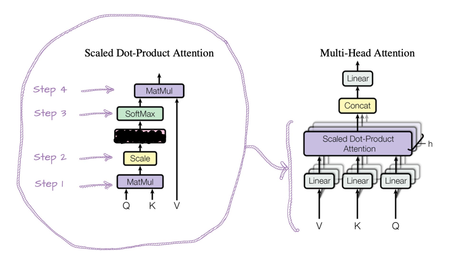
happened once for each word. But in practice, Transformers run multiple attention mechanisms at the same time.

This is called Multi-Head Attention.

Each attention head learns to focus on different types of relationships between words. For example:

• One head might learn to track pronoun references ("it" → "cake"),

• Another might focus on verb-object relationships ("ate" → "cake"),

• Another might pick up sentiment cues ("delicious" → "cake").

By letting multiple heads run in parallel, the Transformer captures a richer understanding of the sentence.

Each head runs the process we described above, and then, all of the heads are concatenated together. Matrix concatenation is literally building wider matrices (capturing more features). For example:

• If each head output is 4-dimensional (d_v = 4),

• And we have 8 heads (h = 8),

• After concatenation, each word's vector becomes 4 × 8 = 32 dimensions.

📢 In this post, we broke down how Transformers actually build meaning — not just by passing embeddings around, but by mixing information from the whole sentence through self-attention.

We walked through:

• How queries, keys, and values are created,

• How similarity is measured,

• Why scaling and softmax are needed,

• And how context vectors are formed through a final weighted aggregation.

All using matrices, intuitive examples, and plenty of visuals to make it concrete.

But now, I would love to hear from you:

• Was this your first real deep dive into self-attention?

• Did the analogy with Netflix movies help you connect the math with real intuition?

• Or maybe you had a small “aha!” moment realising that multi-head attention is not magic — it is just parallel matrix operations?

Drop your thoughts, questions, or even lingering confusions in the comments — I would love to hear how this clicked (or did not!) for you. 👇

If you are interested in more content, here is an article capturing all my written blogs!