Diffusion Models - II: Inside Stable Diffusion

In an earlier post, I discussed basics of diffusion. We built diffusion from thermodynamics to DDPM, demonstrated the coarse-to-fine hierarchy on MNIST, and introduced latent diffusion as the two-stage approach (VAE compression + diffusion in latent space) that made stable diffusion possible. We outlined Stable Diffusion pipeline:

1. Text encoding. The prompt e.g. “a cat sitting on a windowsill, afternoon sunlight” is tokenized and passed through (CLIP) text encoder, producing a sequence of 77 embedding vectors in a 768-dimensional space. These vectors encode the semantic content of the prompt.

2. Latent initialization. A random tensor z_T ∼ N(0,I) is sampled in the latent space (64×64×4). This is pure noise and forms the starting point of the reverse diffusion process.

3. Iterative denoising. For t = T, T-1, …, 1: the U-Net takes the current noisy latent z_t, the timestep t, and the text embeddings c, and predicts the noise component ε^. (Classifier-free guidance amplifies the text-conditional prediction.) The noise is partially removed according to the DDPM update rule, producing z_{t-1}. This is the reverse diffusion process, each step moves the latent slightly closer to a clean, text-consistent image.

4. Decoding. The final clean latent z_0 is passed through the VAE decoder, producing a 512×512×3 image. This single decoding step transforms the abstract latent representation into actual pixels.

But we described these components superficially, avoiding any intricate details. In this post, I’ll talk about some aspects of the pipeline that complete the picture of stable diffusion.

Part I described the U-Net as an encoder–decoder with skip connections. That description is correct but insufficient. The U-Net in Stable Diffusion is a 860-million-parameter network (for SD 1.5; 2.6 billion for SDXL) with a carefully designed internal structure that embodies the coarse-to-fine hierarchy we observed on the Swiss roll and MNIST. A key detail is how the text comes into the architecture and how it steers the generation. Let’s fill in some of the details of how this works.

The text prompt enters the U-Net through cross-attention layers, interleaved with the self-attention layers at the same resolution levels. The mechanism is the core of how language controls image generation, and it is worth understanding precisely.

In standard self-attention, the queries, keys, and values all come from the same source (the image features). In cross-attention, the queries come from the image features, but the keys and values come from the text embeddings:

Each spatial position in the image forms a query that asks: “which parts of the text are relevant to me?” The attention weights form a matrix that maps text tokens to spatial positions. A patch in the upper region of the image might attend strongly to the word “sky.” A patch in the center might attend to “cat.” A patch at the bottom might attend to “windowsill.”

This happens at multiple resolutions. At 8×8, cross-attention handles high-level composition — where subjects go, the overall scene layout. The 64 spatial tokens each attend to 77 text tokens, and the attention pattern effectively assigns each region of the image to a concept in the prompt. At 16×16, cross-attention handles medium-level structure — the shape of the cat, the outline of the windowsill. At 32×32, it handles fine details — the texture of fur, the grain of wood.

The multi-scale nature of this conditioning is part of what makes Stable Diffusion’s prompt adherence effective. The text does not just set a global theme, it guides the generation at every spatial scale. And because cross-attention is applied at every denoising step, the text continuously steers the process from the initial gross composition through the final texture.

There is a beautiful connection to the coarse-to-fine hierarchy from Part I. At early denoising steps (high noise), the U-Net’s predictions are dominated by the deep, low-resolution features. The cross-attention at 8×8 determines where subjects go. At late denoising steps (low noise), the predictions are increasingly influenced by the high-resolution features. The cross-attention at 32×32 determines what textures appear. The temporal hierarchy of denoising (coarse structure first, fine detail last) and the spatial hierarchy of the U-Net (deep layers for global, shallow layers for local) are aligned. And the text conditions both, at every level.

In the previous post, we introduced classifier-free guidance that amplifies text adherence by extrapolating between conditional and unconditional predictions. The formula we used was:

Here w controls adherence to the prompt. Let's understand what this actually does geometrically and why it has the side effects it does.

The Double Forward Pass: At every denoising step, classifier-free guidance requires two forward passes through the U-Net: one with the text conditioning and one without. This literally doubles the compute cost of generation. Every acceleration trick in the Stable Diffusion ecosystem (reduced step counts, distilled models, caching strategies) is partly an attempt to claw back this factor of two.

The Geometry: Think of the noise prediction as a vector in a 16,384-dimensional space (the dimensionality of the latent tensor, 64×64×4). The unconditional prediction ε_θ(x_t, t, ∅) points toward “some clean image” which is the model’s best guess given only the noise level, with no preference for content. The conditional prediction ε_θ(x_t, t, c) points toward “a clean image consistent with the prompt.”

The difference between them ε_θ​(x_t​, t, c) − ε_θ​(x_t, t, ∅) is the purely text-dependent component. It is the part of the prediction that exists only because of the conditioning. Multiplying this component by w > 1 extrapolates beyond the model’s learned conditional distribution, pushing the image further in the direction the text indicates than any training example would warrant.

At w=1: the raw conditional prediction. Images are diverse but sometimes vague, hedging between multiple valid interpretations.

At w=7.5 (SD 1.5 default): sharper and more text-faithful than any single training image. The model is pushed beyond its training distribution in the text-consistent direction. The characteristic “AI look” begins, slightly too vivid, too perfectly composed.

At w=20+: extreme extrapolation. Colors saturate. Edges hyper-sharpen. Textures become repetitive. The image is a caricature of the prompt, pushed so far that naturalness is sacrificed entirely.

The choice of guidance scale is an aesthetic judgment. Lower guidance produces more natural, painterly images with room for the model’s own “interpretation.” Higher guidance produces crisper, more literal results. This diversity versus fidelity trade-off is fundamental. It cannot be eliminated, only navigated.

• SDXL (2023): SDXL stayed within the latent U-Net framework but improved every piece. The U-Net grew from 860M to 2.6B parameters. A second text encoder, producing embeddings in a 1280-dimensional space, was added alongside CLIP. The two sets of text embeddings are concatenated and fed through cross-attention jointly, giving the model a richer textual representation. The native resolution doubled to 1024×1024.

  A refinement stage was introduced which uses a second, smaller diffusion model that reruns a short diffusion process on the output of the base model, sharpening details that the first pass left soft. This improved fine detail (small text, facial features, intricate patterns) substantially.

  The images were noticeably better. But the fundamental architecture was unchanged.

• Stable Diffusion 3 (2024): SD3 made a more radical change. It replaced the U-Net entirely with a Diffusion Transformer (DiT), a pure transformer operating on patches of the latent space. Instead of the U-Net’s hierarchical encoder–decoder with multi-resolution processing, the DiT treats the image as a flat sequence of patches and processes them through a stack of transformer blocks with full bidirectional attention. Image patches and text tokens live in the same sequence, there is no separate cross-attention mechanism. Everything attends to everything.

  This eliminates the U-Net’s inductive bias toward multi-resolution processing, replacing it with the transformer’s more flexible but more data-hungry attention mechanism. DiT models need more data and compute to train, but they scale more predictably and handle complex compositional prompts better.

  SD3 also replaced the DDPM noise schedule with rectified flow — a form of flow matching that transports noise to data along straighter paths, enabling generation in 20–30 steps instead of 50–100.

The conceptual trajectory: the framework has remained stable since DDPM. What changed is the denoising network (U-Net → Transformer), the noise-to-data path (stochastic SDE → straight-line flow), and the text encoder (CLIP → T5-XXL). The core idea (learn the score, reverse the process) is unchanged.

In this section, I describe an experiment where I take Stable Diffusion and teach it a new visual style. The style is Ernst Haeckel’s Kunstformen der Natur (1904). Radiolarians, jellyfish, ferns, and siphonophores rendered in meticulous copperplate lines, stippled shading, and the tonal palette of a 19th-century lithographic press. Science and art inseparable on the plate.

We fine-tune using LoRA (Low-Rank Adaptation) so that prompts like “a cat sitting on a windowsill” or “the solar system” produce images that look like they belong in a 19th-century encyclopedia.

The choice is deliberate. Haeckel’s illustrations have a strong, instantly recognizable visual signature, you know a Haeckel plate at a glance. The style is consistent across 100 plates: the same linework, the same tonal range, the same compositional language of radial symmetry and dense taxonomic arrangement. The images are firmly in the public domain. And the aesthetic is beautiful enough that the experiment is worth doing for its own sake.

More importantly, Haeckel’s style is complex enough to stress-test LoRA’s capacity. It is not a simple texture or color filter. It involves multiple interacting visual elements: the weight and rhythm of copperplate lines, the density gradients of stippled shading, the interplay of positive and negative space, the specific conventions for rendering transparent biological structures, the muted lithographic palette. A model that learns this style has learned something compositional, not just a surface transformation.

We start with 35 plates downloaded from Wikimedia Commons: Acanthometra, Ascidiae, Bryozoa, Calcispongiae, Discomedusae, Siphonophorae, and so on.

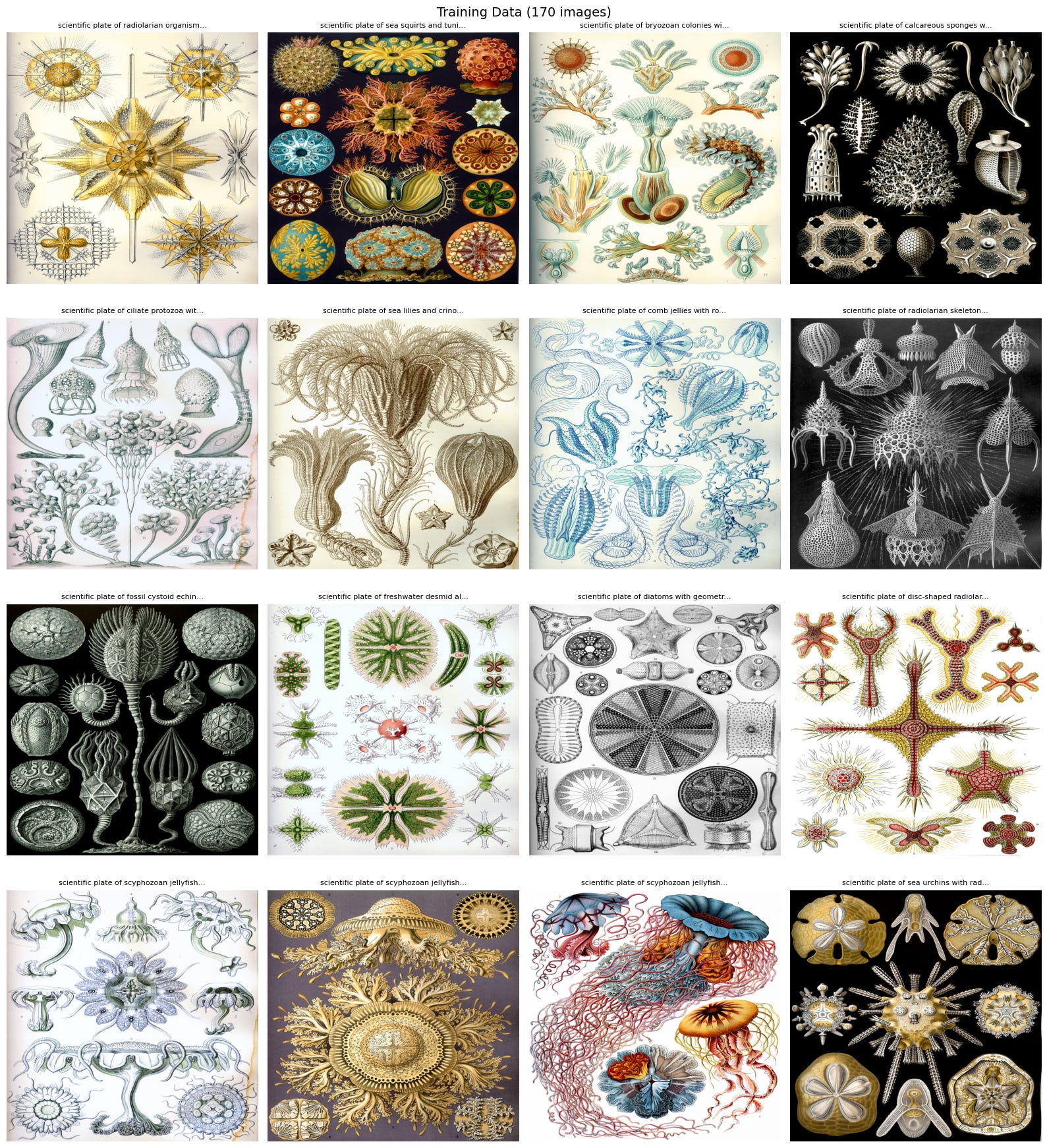
Each image is paired with a descriptive caption ending in a trigger phrase: “vintage scientific engraving.” The trigger is the textual anchor for the style. During training, the model learns to associate the trigger with the visual characteristics of the training images. At generation time, including the trigger activates the learned style via the cross-attention mechanism.

The captions matter more than they might seem. A generic caption like “scientific plate of discomedusae” teaches the model little about the visual content. A descriptive caption like “scientific plate of scyphozoan jellyfish with broad translucent bell, flowing oral arms, and trailing tentacles against dark background” creates much richer associations. The cross-attention layers learn to associate specific words (”translucent bell,” “flowing oral arms”) with specific visual patterns (the hatching technique for transparency, the curved parallel lines for flowing forms). Better captions produce better style transfer because they give the cross-attention mechanism more to work with.

To extract more training signal, we crop each plate into four quadrants. Haeckel’s plates are densely packed — a single plate of Discomedusae contains eight jellyfish, each with distinct morphology. The crops teach the model the fine linework at a detailed level, not just overall composition. From 35 plates, we get approximately 175 training images.

The U-Net has 860M parameters (SD 1.5) or 2.6B (SDXL). Fine-tuning all of them on 175 images would overwrite the model’s general visual knowledge with an overfitted memory of 35 plates.

LoRA (Hu et al., 2021) freezes every original weight and adds a small, trainable perturbation to each attention matrix W:

where

With r=16, we train approximately 6.5 million parameters, less than 1% of the model.

Why does this work? Artistic styles live in a low-dimensional subspace of the model’s behavior. The model already knows anatomy, perspective, composition, lighting. It does not need to relearn any of this. It only needs to adjust the rendering. LoRA’s low-rank matrices are precisely the right tool: they can express a coherent global shift in output distribution without the capacity to memorize individual training images.

• Base model: SDXL (1024×1024, 2.6B U-Net)

• Dataset: 35 plates + ~140 crops ≈ 175 images

• LoRA rank: 16, all attention projections

• Learning rate: 2 × 10⁻⁵, cosine schedule, 200-step warmup

• Steps: 2,000 (~45 epochs)

• Precision: bfloat16

• Gradient accumulation: 4 (effective batch size 4)

• GPU: A100 (40GB), ~3 hours

• Checkpoints: every 500 steps with evaluation grids

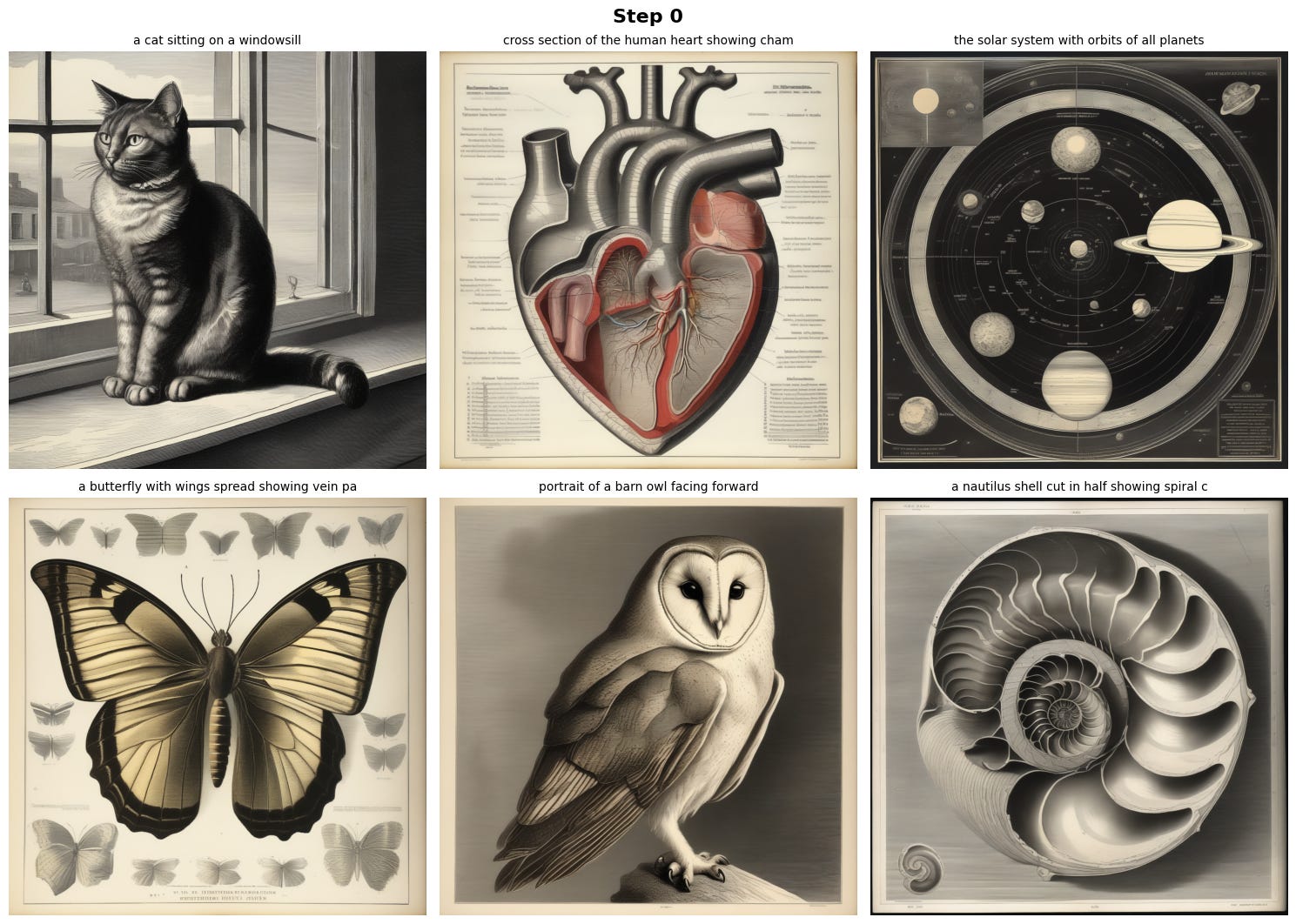
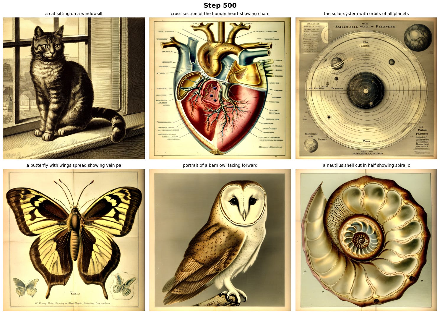
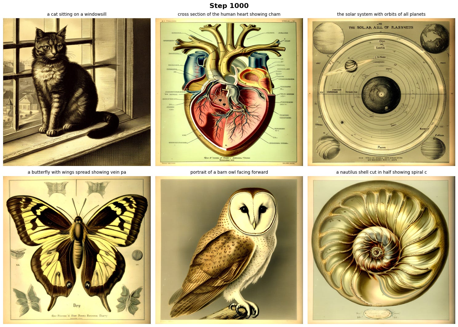
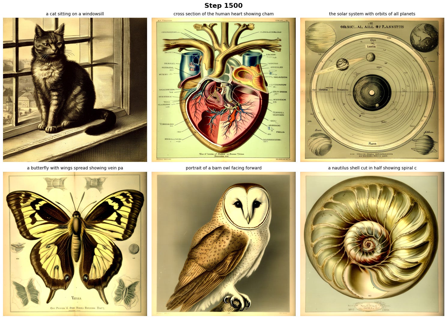
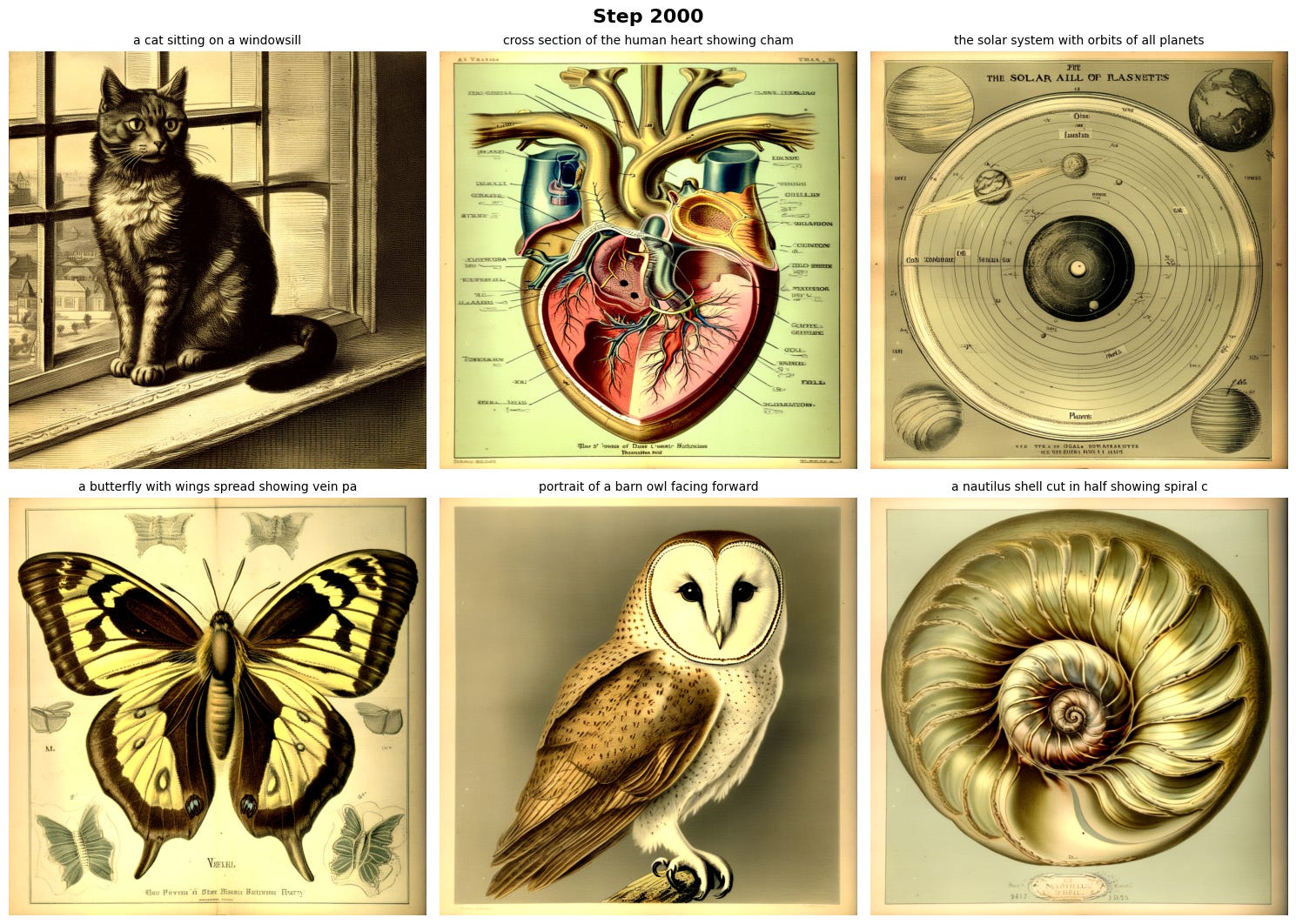
We generate the same six prompts a cat, an anatomical heart, the solar system, a butterfly, a nautilus shell, a barn owl) at every checkpoint using the same random seed.

Step 0 (untrained LoRA): base SDXL output. Photographic, no engraving aesthetic.

Step 500: tonal shift begins. Colors desaturate toward sepia and slate. Early line texture in shadows, but forms still photographic. The model has learned the low-frequency statistics of the Haeckel distribution (palette) but not yet the high-frequency ones (linework).

Step 1,000: clear engraving character. Crosshatching appears in shadows. Backgrounds shift to uniform lithographic tones. Subjects maintain anatomical accuracy but are rendered in ink rather than light.

Step 1,500: style fully established. Fine stippling in gradients. Copperplate line weights in contours. Images look like 19th-century encyclopedia plates, depicting subjects Haeckel never illustrated. This is LoRA working as designed: pretraining knowledge preserved, rendering redirected.

Step 2,000: slightly more refined, diminishing returns. The cosine schedule has nearly decayed the learning rate to zero.

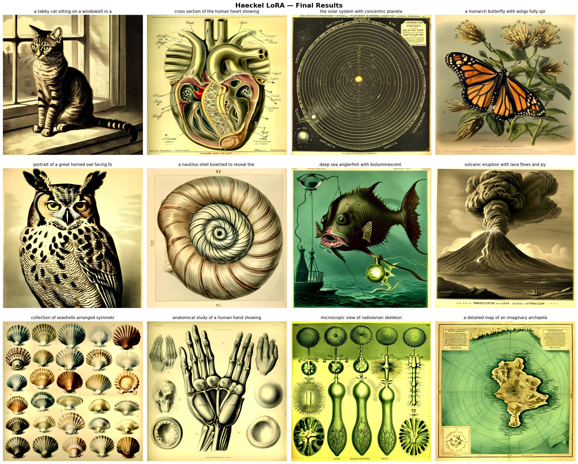
At full quality — 50 denoising steps, guidance scale 6.0, trained LoRA active:

The transformation is not a texture overlay. The model has learned the compositional logic of Haeckel’s plates: radial symmetry for marine organisms, bilateral symmetry for vertebrates, the way negative space frames specimens, the gradation from dense crosshatching in shadows to open stippling in highlights. It has learned the tonal palette (warm sepia backgrounds, deep black contours, muted hand-tinted greens and blues) as well as the line vocabulary (tight parallel hatching for smooth surfaces, irregular stippling for organic texture).

None of this was explicitly programmed. The model inferred the style’s internal structure from 35 plates and less than 1% of its parameters, guided by the same training objective we introduced in Part I.

Part I built the theory: Langevin dynamics, score matching, DDPM, the coarse-to-fine hierarchy, and the introduction to latent diffusion. This post went inside: the cross-attention mechanism mapping language to spatial features, the geometry of classifier-free guidance, the evolution from U-Nets to Transformers.

And we closed the loop with an experiment. The Haeckel LoRA is a small experiment (35 training images, a few hours on one GPU) but it exercises the full stack. The DDPM objective runs in the VAE’s latent space. Cross-attention associates the trigger phrase with the visual style. Classifier-free guidance amplifies this at generation time. LoRA adapts the attention layers without disturbing the model’s pretraining. And the coarse-to-fine hierarchy we first saw on a 2D spiral now produces stippled jellyfish and crosshatched owls at 1024×1024.

The field continues to evolve. Flow matching is replacing classical diffusion. Diffusion Transformers are replacing U-Nets.

And a question I would like to explore next: what happens when you try to diffuse something discrete e.g. language, protein sequences, molecular graphs? Can you add noise to a word? In Part III, we confront that frontier.

If you find this post useful, I would appreciate if you cite it as: