ML and LLM Inference Latency: 10 techniques every AI/ML engineer should know

Hi there 👋 ,

There’s a moment in every AI/ML engineer’s career when latency stops being a model problem and becomes a system problem.

It usually happens around the time the first wave of real traffic hits production. The model runs fine on your laptop. Benchmarks look healthy in staging. Then you ship, p99 latency starts climbing, inference costs balloon, and you spend the next two weeks chasing optimizations that have nothing to do with the model’s weights.

The model is one component in a longer chain. Network round trips, request serialization, queueing, batching strategy, memory layout on the GPU, the precision of the weights, whether you’re recomputing things you’ve already computed: all of these matter, and most of them are invisible until something breaks.

This post is the playbook I wish I’d had. It covers ten techniques across both classical ML and LLM serving, organized around what each technique actually does to the bottleneck. The mental model comes first, because without it, the techniques are just a list.

Note: at the bottom we mention a decision framework that you should know and utilize it in your upcoming interviews or while building production systems.

Before any technique is worth discussing, three distinctions need to be in place. Skip these and you’ll spend weeks on the wrong optimization.

Latency is how long a single request takes from arrival to completion.
Throughput is how many requests the system can process per second across all users.

They’re related but they pull in different directions. Batching multiple requests together improves throughput, because the GPU can process them in parallel. But the first request in the batch has to wait for the others to arrive before processing starts, so its latency goes up.

Most of the techniques in this post are honest about which they optimize. A few improve both. Several improve throughput at a small cost to single-request latency, which is fine under heavy load (when latency would otherwise collapse from queueing) but a bad trade at low load. Knowing which is which is the difference between solving your problem and making it worse.

For classical ML models (a fraud classifier, a recommendation ranker, a vision model), the latency budget breaks down roughly into preprocessing, the forward pass, and postprocessing. Most production ML systems are bottlenecked either on the forward pass itself or on I/O around it: loading features from a database, fetching embeddings from a cache, hitting an external service for enrichment.

The forward pass is usually compute-bound for vision and audio models and memory-bound for tree-based models that don’t fit in cache. The optimization space is relatively narrow: make the model smaller, make the math faster, batch better, cache more, get the I/O off the critical path.

LLMs are a different shape of problem entirely.

An LLM inference call has two distinct phases that behave nothing like each other.

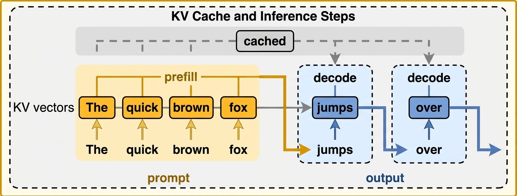
The first is prefill, where the model processes the entire input prompt in parallel. Prefill loads the model weights once, runs the prompt through every layer, and produces the first token along with a cache of intermediate state. Prefill is compute-bound. For a 4K-token prompt on a modern GPU, prefill takes a few hundred milliseconds.

The second is decode, where the model generates output tokens one at a time. Each new token requires loading the model weights from GPU memory all over again. The math per token is small (a single forward pass on a single token), but the data movement is enormous: gigabytes of weights loaded for each token generated. Decode is memory-bound. The bottleneck isn’t the GPU’s compute, it’s the speed at which it can read its own memory.

This split is the single most important thing to internalize about LLM latency. Optimizations that target prefill don’t help decode, and vice versa. FlashAttention helps both because it touches the attention computation in both phases. Speculative decoding only helps decode. Prompt caching only helps prefill (more on this below) If you don’t know which phase your bottleneck lives in, you can’t pick the right tool.

This phase split also dictates how latency is measured. Two numbers matter:

Time to first token (TTFT) is how long the user waits before seeing any output. TTFT is dominated by prefill. For a streaming chat product, TTFT is what users perceive as “how long does it take to start responding.”

Time per output token (TPOT) is the gap between successive tokens. TPOT is dominated by decode. Once the response has started, TPOT determines whether it feels fast (50+ tokens per second) or laborious (10 tokens per second).

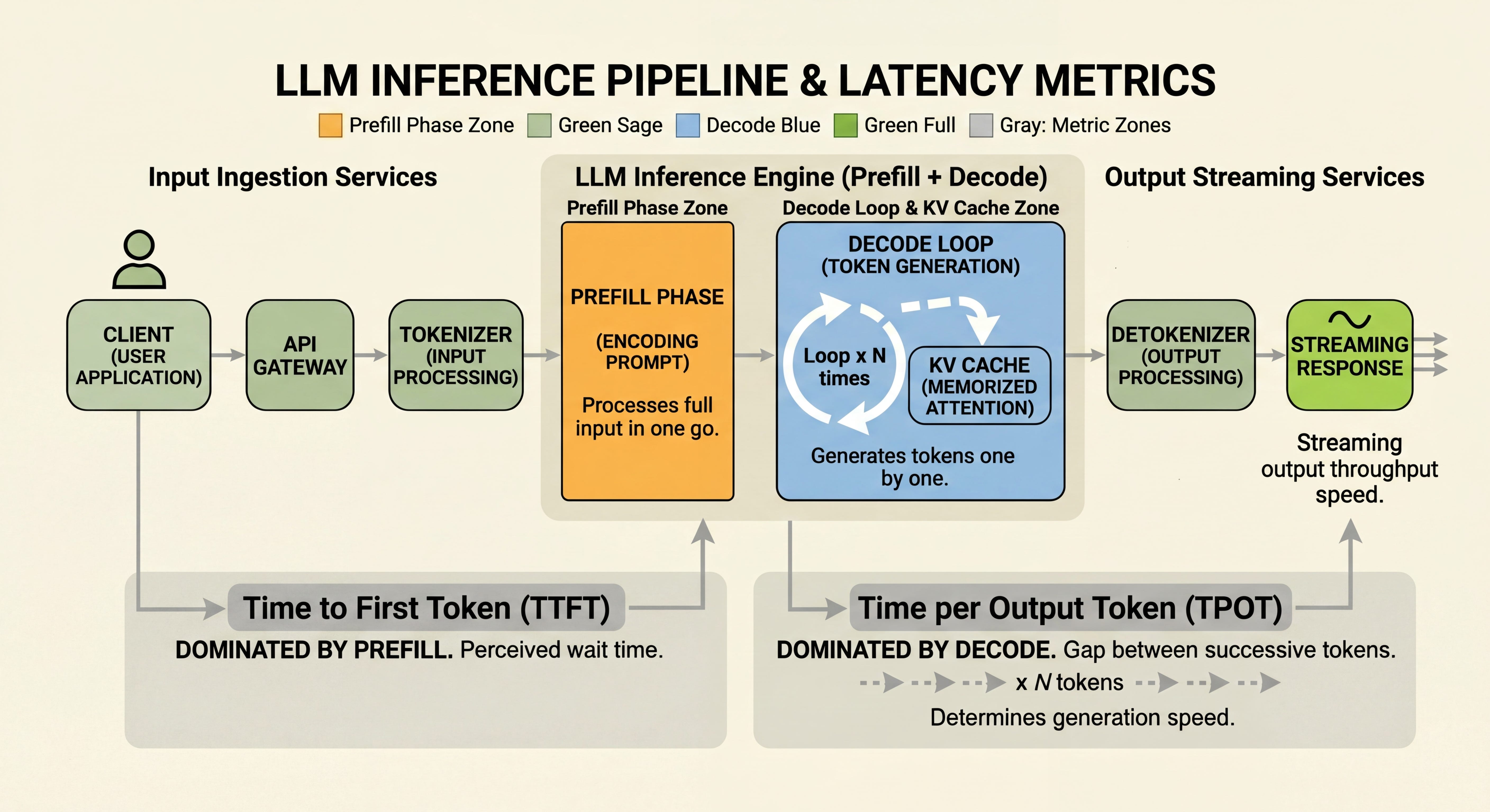
End-to-end latency is roughly TTFT plus TPOT multiplied by the number of remaining output tokens. For a chatbot generating short answers, TTFT is everything. For a code-completion tool generating multi-paragraph diffs, TPOT dominates. Knowing which metric your product needs to move is what makes the difference between picking the right optimization and picking the wrong one.

The best AI engineers I know didn't learn from courses. They learned by watching how real teams ship in production.
This Summit is a great place to invest a few hours if you're working on enterprise AI systems.

Register for Free

These five apply to both classical ML and LLM serving. They’re the foundation, and most teams under-use them before reaching for fancier tricks.

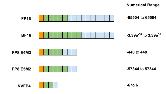
Model weights have traditionally been stored as 32-bit floating point numbers, though most modern LLMs are now released in 16-bit (BF16 or FP16) by default. Quantization pushes this further, compressing weights into 8-bit or 4-bit representations. Storing weights in 4-bit instead of 32-bit reduces the memory footprint by a factor of eight, which directly accelerates the memory-bound parts of inference because there’s less data to move.

In practice, the latency win is biggest for LLM decode (which is memory-bound) and smaller for prefill or for compute-bound classical ML models.

The catch is accuracy. Aggressive quantization to 4 bits can degrade output quality, especially for smaller models. Mixed-precision approaches (using fp16 for most operations and fp32 selectively for sensitive ones) are usually the safe starting point. For LLMs, GPTQ and AWQ are the two standard algorithms for 4-bit weight quantization, paired with file formats like GGUF (used by llama.cpp) for distribution. Most production teams now quantize as a default rather than an optimization.

Most large neural networks are over-parameterized. Many weights contribute almost nothing to the output. Pruning identifies which connections are doing the least work and removes them, typically reducing model size by 10 to 25% with minimal accuracy loss. Structured pruning (removing whole channels or layers) is friendlier to hardware than unstructured pruning (removing individual weights), even though it tends to compress less.

Distillation goes further. It trains a smaller “student” model to imitate the outputs of a larger “teacher” model. The Phi family is a well-known case, drawing heavily on synthetic data partly distilled from larger models, and the smaller Llama 3.2 variants (1B, 3B) were distilled from larger Llama checkpoints. Done well, a distilled smaller model can match or beat a model two to three times its size on the tasks it was trained for, while running substantially faster. (This is also how many of the opensource LLMs are being gathering training data - source)

Both techniques apply equally to classical ML and LLMs. The cost is offline: you do the work once during training and benefit from it on every subsequent inference.

A model written in PyTorch is a Python program full of operator dispatch overhead. Compilers like TensorRT, ONNX Runtime, and torch.compile take that program and transform it into hardware-specific code that fuses operations, reduces memory transfers, and exploits the GPU’s specific architecture.

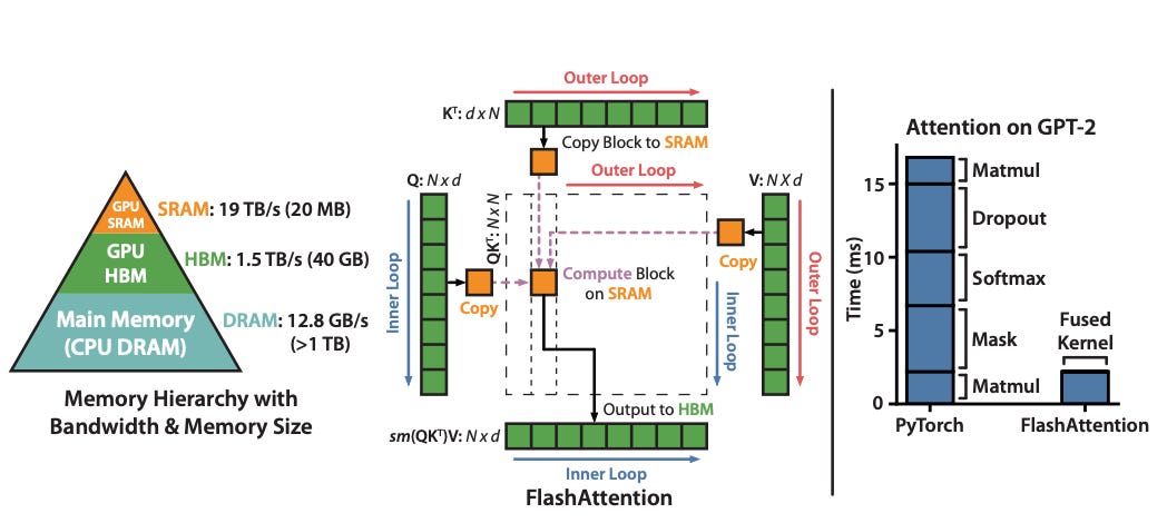
The most famous example for transformers is FlashAttention, which restructures the attention computation to work on small tiles that fit in the GPU’s fast SRAM rather than constantly shuttling data to and from slower high-bandwidth memory. For most modern GPUs, FlashAttention delivers 2 to 4x faster attention with no accuracy loss, with the biggest wins in prefill where sequences are long. Modern variants (FlashDecoding and FlashAttention v3) extend the same ideas to the decode phase. It’s used under the hood by almost every serious LLM serving stack.

The general rule: compile your model for the hardware it’s actually going to run on. The default PyTorch eager-mode execution is convenient but leaves significant performance on the table.

Caching is the cheapest optimization that exists, and most teams under-use it. There are three distinct flavors worth distinguishing.

1. Request-level caching stores the full response for an exact input match. If 200 users ask “how do I reset my password,” you compute the answer once. Redis in front of your inference endpoint covers this in a few hours of work.

2. Semantic caching matches similar inputs using embedding similarity rather than exact equality. “How do I reset my password” and “I forgot my password, how do I reset it” return the same cached response. This requires a similarity threshold and an embedding model, but it dramatically expands cache hit rates for natural-language queries. The risk is false positives, where two questions that look similar by embedding actually need different answers, so the threshold needs careful tuning.

3. Prompt caching is LLM-specific and recently became available through the Anthropic, OpenAI, and Gemini APIs. It caches the KV computations for a static prefix. If your application sends the same 8,000-token system prompt with different user messages, prompt caching computes the prefix once and reuses it across requests.

   For RAG and long-context applications, this often delivers a larger TTFT reduction than any other single technique. If you’re calling a hosted LLM API and you’re not using prompt caching for repeated prefixes, you’re paying full price on every call for work the provider has already done.

The most reliable latency optimization is the one engineers resist the most. A 7B model serves several times faster than a 70B model and fits on hardware the 70B doesn’t (a single A100 vs a multi-GPU setup with sharding overhead). A fine-tuned smaller model often beats a generic larger one on the specific tasks your product cares about.

The blocker isn’t usually technical. It’s psychological. Engineers want to use the best available model because that’s what the benchmarks reward and what the team Slack channel celebrates. But for a customer support classifier, a translation step in a pipeline, or a function-calling decision, GPT-5 or Claude Opus is overkill. A distilled 3B model with a focused fine-tune will outperform on those tasks at a fraction of the cost and latency.

The hard part is benchmarking. You need real evaluation datasets to know when a small model is good enough and when you genuinely need a larger one. Without those, the path of least resistance is to default to the biggest model and pay for it forever.

These four are specific to transformer-based LLMs and don’t really apply to classical ML. They also happen to be where most of the recent serving innovation has happened.

In a transformer, every token has a Key (K) and Value (V) representation that gets used in attention computations. Without caching, generating the 100th token would require recomputing K and V for all 99 previous tokens. KV caching stores these matrices after they’re first computed and reuses them, so generating each new token only requires fresh computation for that one token.

KV caching is the foundation of practical LLM serving. Every modern inference engine implements it. Without it, every new token would require redoing all the projection work for every previous token, so generating a 1,000-token response would do roughly 500 times more work than necessary. Long contexts would be prohibitively expensive.

The cache itself can also be compressed. Techniques like KV cache quantization (TurboQuant) reduce the cache to roughly 3 bits per value, allowing much longer contexts to fit in the same GPU memory. Prompt caching, mentioned above, is essentially KV caching extended across requests for static prefixes. The KV cache is the single most important data structure in LLM serving, and most production-readiness questions about latency end up being questions about how it’s managed.

A naive KV caching implementation reserves a fixed-size memory block per sequence, sized for the maximum possible context length. If a user has a short conversation but the system reserved space for a 32K-token context, most of that GPU memory sits idle. With many concurrent users, this waste compounds and limits how many requests the system can serve in parallel.

PagedAttention solves this by allocating the cache in small fixed-size “pages” (typically 16 tokens each), allocated dynamically as sequences grow. Memory is no longer reserved upfront; it’s borrowed as needed and returned when sequences finish. The result is that the same hardware can serve 2 to 4x more concurrent requests with no change in single-request latency.

PagedAttention is the headline optimization in vLLM, which has become the most common LLM serving engine in production. If you’re running your own inference cluster and you’re not using PagedAttention, you’re likely paying for two to four times more GPU capacity than you actually need. Note that this is fundamentally a throughput optimization. It doesn’t make a single request faster, it lets you serve more of them in parallel without buying more hardware.

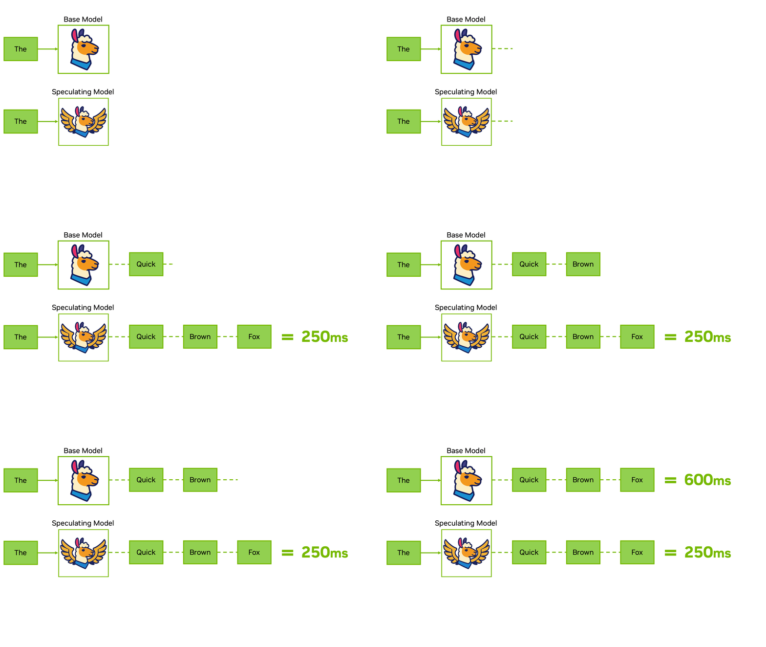
Many tokens in an LLM’s output are easy to predict. The token after “Generating sentences with LLMs is” is almost certainly “expensive” or “slow” or some similar adjective. A small model can guess these correctly most of the time, in a fraction of the compute cost of running the full model.

Speculative decoding exploits this. A small “draft” model proposes the next 5 to 10 tokens. The large model then runs a single forward pass to verify all of them at once, exploiting the fact that transformer outputs include probability distributions for every position in parallel. If the large model agrees, all those tokens are accepted in the time it would have taken to generate one. If the large model disagrees at some position, the speculation is truncated there and the large model’s choice replaces it.

In practice, speculative decoding delivers 2 to 3x faster decode for tasks where token-by-token prediction is relatively easy: summarization, code completion, structured output. Creative writing benefits less because more tokens are genuinely hard to predict. The technique only affects TPOT; it does nothing for TTFT, since prefill already runs in parallel.

In a naive batched system, you collect a batch of requests, run them all together, wait for the longest one to finish, and only then start the next batch. Because LLM outputs vary wildly in length (some users get 50-token answers, others get 4,000-token answers), short requests end up waiting through long ones, and GPU slots sit idle while a few stragglers finish.

Continuous batching (sometimes called in-flight batching) treats the batch as a moving slot pool rather than a fixed group. As soon as any request finishes, a new request can take its slot, even while other requests in the batch are still generating. The result is much higher GPU utilization and dramatically higher system throughput, often 10 to 20x what naive batching delivers.

Be honest about what this technique does. It primarily improves throughput, not single-request latency. Under low load, continuous batching might add a small TTFT cost while the system waits to fill batch slots. Under high load (which is when latency actually starts to suffer in production), continuous batching is what keeps the system responsive instead of collapsing into a queue. It’s a throughput optimization that protects latency under pressure.

The model is one component in a longer chain. Network round trips, request serialization, queueing, preprocessing, and result formatting all sit between the user and the GPU. None of them get optimized by FlashAttention or quantization. They get optimized by paying attention to the serving path itself.

The biggest wins here come from a few specific tactics. Use gRPC instead of HTTP for service-to-service calls, since the binary protocol cuts serialization overhead substantially compared to JSON over HTTP/1.1.

Run preprocessing (tokenization, embedding lookup, retrieval) asynchronously so the GPU isn’t waiting on CPU work. Place inference servers in regions close to your users to cut network round-trip time, especially for chat products where users feel every 100ms.

For user-facing chat products, the most impactful serving-layer optimization is streaming. Strictly speaking, streaming doesn’t reduce latency at all. The total time to generate a response is unchanged. What it changes is perceived latency. A response that appears token-by-token starting at 200ms feels much faster than one that appears all at once at 5 seconds, even though the second one technically delivers more content per second once it starts. Streaming is the difference between a chat product that feels alive and one that feels broken.

Most teams underinvest in the serving path because it’s less interesting than model-level optimization. That’s a mistake. A 50ms improvement in serialization overhead, applied to every request, often saves more aggregate latency than a 10% speedup in the model itself.

None of this matters if you don’t know which lever to pull. Most teams spend weeks on the wrong optimization because they didn’t diagnose the bottleneck first. Here’s how to map symptoms to techniques.

If TTFT is too high. The bottleneck is prefill. Reach for prompt caching first, especially if your application has long static prefixes (system prompts, retrieval context, few-shot examples). Add FlashAttention if your serving stack doesn’t already use it. Consider a smaller model for the prefill-heavy cases, since you can route different requests to different models based on their needs. Make sure prefill is running on hardware with enough compute, since prefill is compute-bound and benefits from higher-end GPUs.

If TPOT is too high. The bottleneck is decode, and decode is memory-bound. Quantize the model so there’s less data to move per token. Add speculative decoding if the task allows it (summarization, code, structured output). Consider KV cache quantization for long contexts. The “use a smaller model” lever applies here too, because smaller models have less weight data to load per token.

If throughput collapses under load. You’re queueing. Continuous batching and PagedAttention are both designed for exactly this scenario. Add more replicas (autoscale on inference queue depth, not CPU utilization). Make sure your load balancer uses inference-aware metrics rather than round-robin, since LLM request costs vary wildly based on input and output length.

If costs are too high. Almost everything in this post helps. The biggest wins are quantization, distillation to a smaller model, and prompt caching for repeated prefixes. Smaller models scale all three of cost, latency, and throughput in the same direction, which is rare and worth exploiting when you can.

Match the technique to the symptom. Optimization without diagnosis is how teams burn six weeks on a 10% improvement when a 60% improvement was sitting in the next layer up.

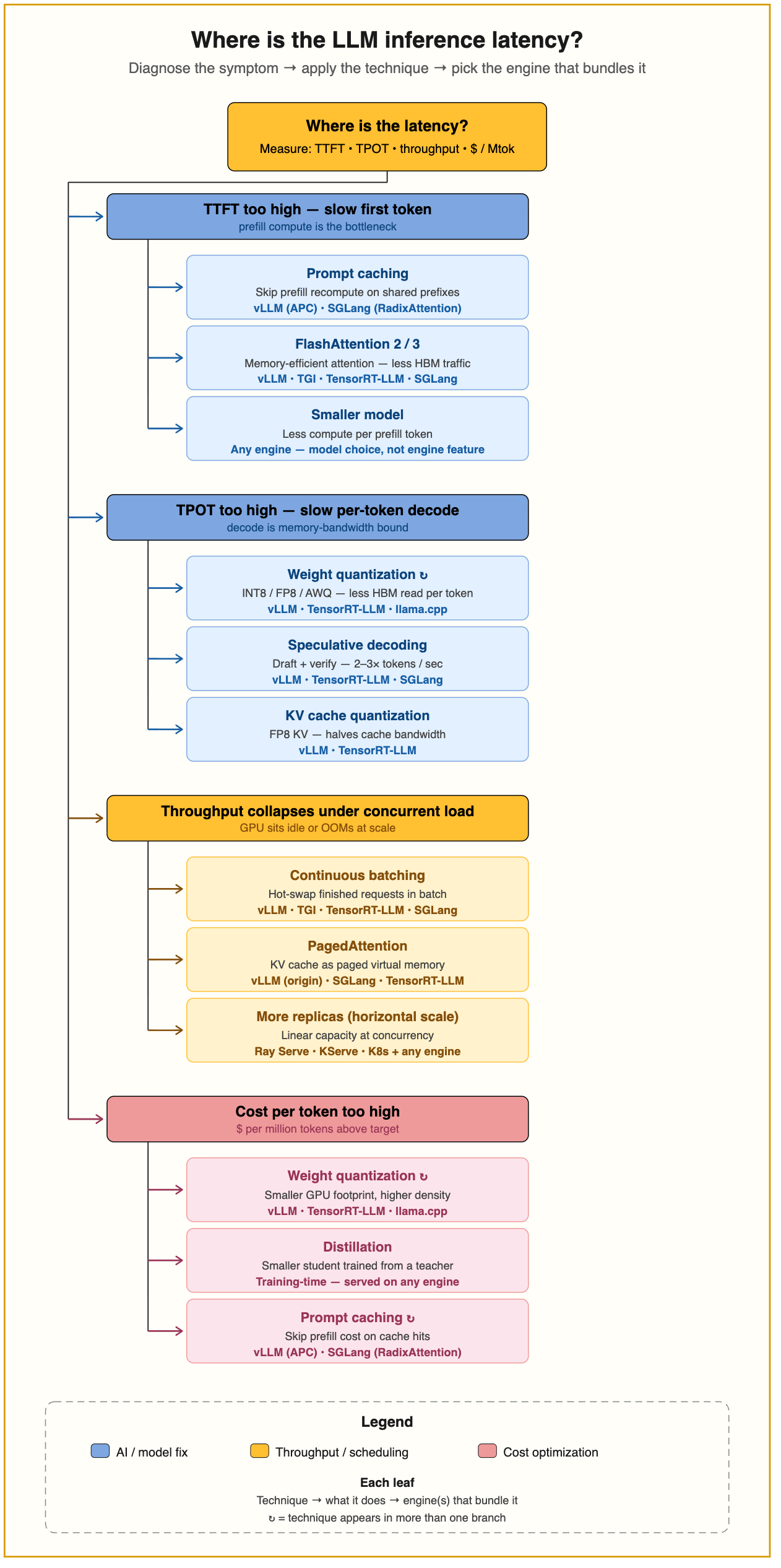
You don’t implement most of these techniques yourself. You pick an inference engine that bundles them.

vLLM is the most common starting point for production LLM serving. PagedAttention, continuous batching, prefix caching, and a sane API. Start here unless you have a specific reason not to.

TensorRT-LLM is NVIDIA’s serving stack. Faster than vLLM on NVIDIA hardware if you’re willing to invest in the compilation step, but with more operational complexity.

SGLang is a newer entrant with strong performance on structured generation and constrained decoding. Worth evaluating if your workload is mostly JSON output or function calling.

TGI (Text Generation Inference) is HuggingFace’s serving stack, well-suited to teams already in the HF ecosystem.

llama.cpp is the canonical option for quantized inference on consumer hardware or CPU. If you’re running models locally or on edge devices, this is where you start.

For classical ML, the equivalents are Triton Inference Server (NVIDIA’s general-purpose serving platform) and Ray Serve (for distributed serving across CPU and GPU).

We hope this was useful, and an important thought:

None of these techniques is exotic. Most are sitting inside vLLM or TensorRT-LLM waiting to be turned on. The hard part isn’t the optimization, it’s knowing which one to reach for. Diagnose first, optimize second.

The next time your model runs slow, the question to ask is which phase the time is going into and whether the bottleneck is compute or memory. Once you know that, the technique picks itself.

Until next time.

If you enjoyed this read? do share it with your colleagues and team :)

Share