Branching into Performance

At the lowest level, all software can be decomposed into individual machine executable instructions that are processed by the CPU. The vast majority of individual instructions are generally broken down into a few categories

• Arithmetic instructions (add, multiply, xor, etc)

  • Separately includes floating point operations

• Memory access instructions (load, store, move)

• Control flow instructions (call, jump, return, etc)

  • These change control flow, and can be either conditional or unconditionally

While there are some additional nuances, this is in general a high level view of everything going on within a CPU. We’re going to be focusing on the control flow for this article, specifically talking about conditional control flow, its performance implications and how to mitigate in certain circumstances.

Control flow is central to software. Any time a function is called, an if statement is checked, a for loop runs or code returns out of a function, there is some control flow that tells the CPU which set of instructions to execute. Consider a basic C++ program

This program takes in some number of arguments, then exits with the exit code equal to the number of arguments squared. The generated assembly for this is as follows1

The generated assembly for square also reflects this new change

We now have a new branching instruction that changes our control flow in a data dependent way. After the initial setup of rbp and rsp, we now have a new cmp or compare instruction, checking our input against the constant 0. That is followed by the jge (jump greater or equal) instruction. This says that if the result of the prior comparison sets the greater or equal flag to true, we should jump to the label LBB0_2, where we do our multiplication. However if that flag was not true and our value was less than 0, we continue to move the literal 0 into the stack, then unconditionally jump to LBB0_3 where we process the teardown and return from the function.

Note that unlike in our simple branchless case, we cannot tell from looking at the program what the sequence of instructions to be executed will be, since we will either execute a store of 0 or a multiplication depending on the data we are provided.

The reason the introduction of conditional branches impacts software performance is due to the instruction pipelining that exists in all modern CPUs. While it seems from looking at the assembly that each instruction executes in a single step, it is actually broken down into various sub operations. Typically these are instruction fetch, instruction decode, execution, memory access and register writeback, though individual architectures can and do have different and potentially deeper pipelines. Once we have this pipelined architecture, we can greatly improve the throughput of instructions in a best case scenario. While instruction 0 is executing, the CPU could be decoding instruction 1 and fetching instruction 2. Indeed in the best case in our five stage pipeline, we could be getting up to 5 instructions per cycle if our pipeline were completely filled.2

While this simplified pipelined system seems fantastic, giving us 5 times the performance of a non-pipelined CPU, there is a major caveat in the form of branches. As noted above, if instruction 0 is executing we could already be in the process of handling instructions 1 and 2. However that is only the case if we know what the next two instructions are. If instruction 0 is a branch, we don’t know until it is evaluated what the next instruction to fetch is, so we end up with a bubble in our pipeline, degrading performance.3

Since our CPUs are highly pipelined, and any bubble in the pipeline causes degraded performance and idle hardware, improving the performance of branches can go a long way to increase the speed of execution for programs. Consider a for loop, which must incur a branch on every iteration to check if the loop is completed

In this loop, we simply sum up the numbers from 0 to nelems, however at each iteration of the loop, we need to check if i is less than nelems before continuing. If we were using a naive pipelined CPU, we would execute our cmp, then jge instruction, then have to wait until the result of that instruction was known before being able to fetch and decode the next instruction. If it took until after the execute portion of the instruction was completed to know which next instruction to fetch, we’d be wasting 2 cycles per iteration of this loop, giving us performance well below our theoretical 5 IPS.

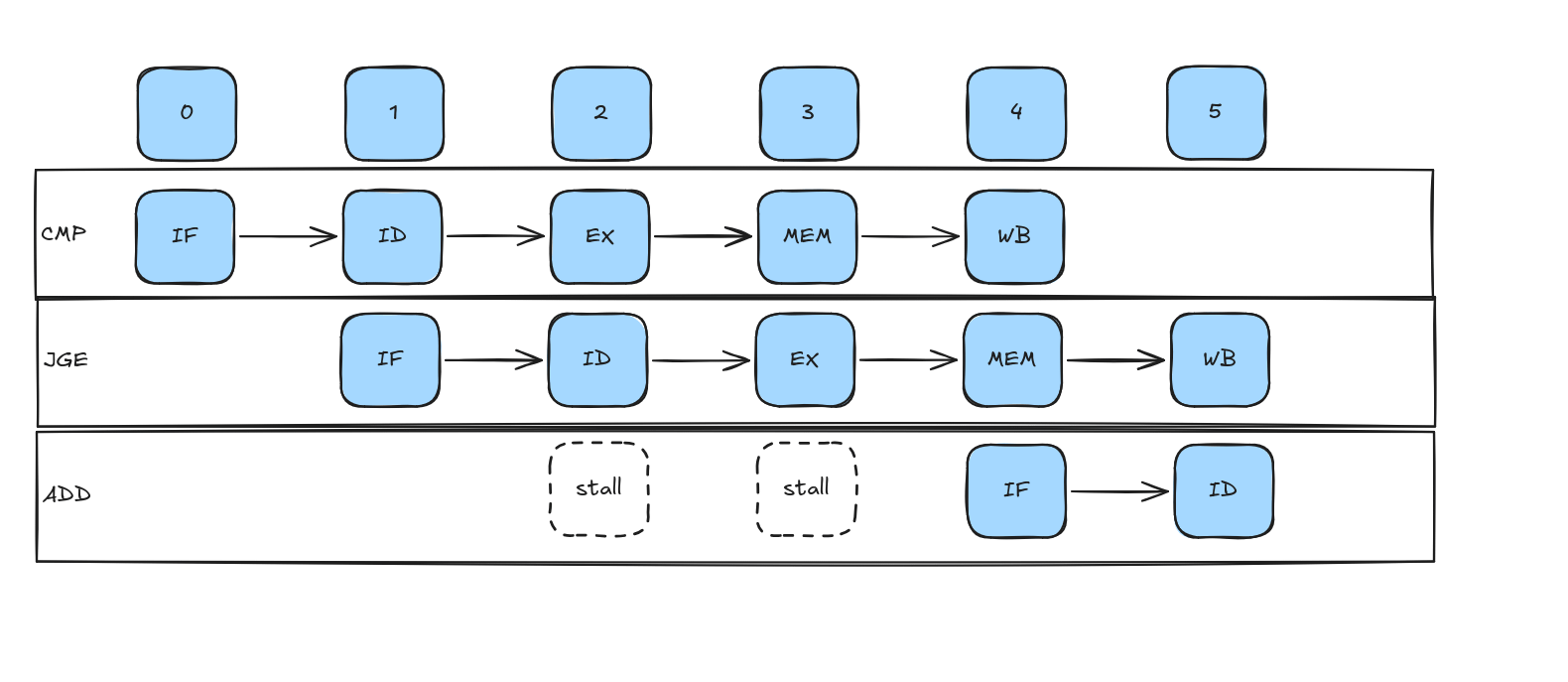
In order to get around this, all modern CPUs ship with branch predictors that allow them to speculate which branch will be executed. These units make a prediction about which branch to take, then the hardware starts executing that branch before the result of the cmp function is known. If the prediction was correct, CPU is already down the processing stream of the instructions and we didn’t have any bubble in the pipeline. However if the prediction was incorrect, it cannot appear as if the branch was actually taken, so anything from the cmp onward has to be flushed out of the pipeline and the CPU needs to go back and restart from the jump instruction. This misprediction can be quite costly.

Fortunately in many programs, branches can be relatively well predicted. In our above summation function, our branch of whether to continue the loop will be quickly learned to predict “branch taken”. Only at the very last iteration of the loop will this prediction be incorrect requiring a pipeline flush, so assuming our loop is executed for a sufficient number of iterations, we should expect an average of nearly 5 instructions per cycle.

To look at what happens when branching goes wrong, we’re going to build up a slightly more complex example to demonstrate. Suppose we have some set of objects, each one of which is either valid or invalid, and has a size, this is represented by the following class

We then have a function to sum up the size of a large collection of objects, only including the size of those objects which are valid. Our first attempt to write this function would be as follows

I’ve then hooked up Google Benchmark to run a large vector of 100,000 objects, each initialized with a random size and a provided fraction of objects to randomly construct as “valid”

Running with a valid fraction ranging from 0.0 to 1.0, we can see how our data dependency impacts our performance dramatically. Plotting out the times, we see the following graph

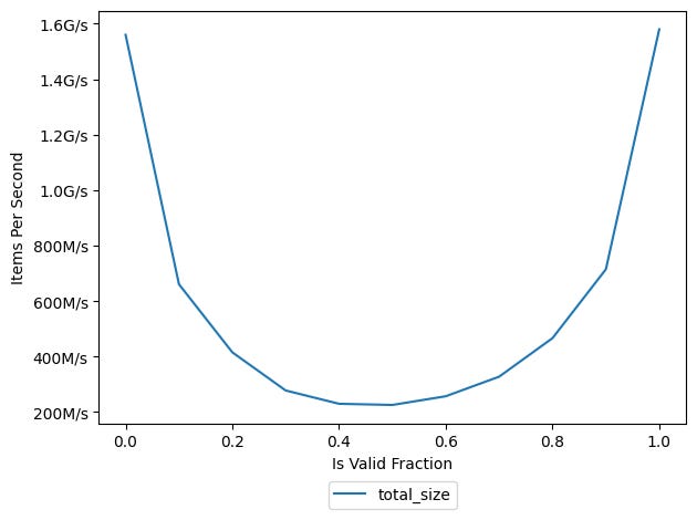
When we start out with all objects being invalid, we’re able to process nearly 1.6 billion objects per second, however as we increase the fraction of objects that are valid, our performance quickly degrades. We reach a nadir of just over 220 million objects per second when half the objects are valid, a mere 14% of the performance when we had all objects being invalid. As we increase our percentage beyond 50%, we recover performance until at 100% of the objects being valid, we’re back to almost the exact same performance as with 0% of the objects being valid.

Let’s dive deeper into why our performance degrades so sharply as the distribution of our data changes. For this, we’re going to use the perf tool, which measures various hardware counters to understand what’s going on in our program at runtime. Two of these counters are of particular interest for our discussion here, namely the branches and branch-misses counters which measure how many branches our program encounters, and how many are mispredicted. Running this on our benchmark program with a 0.0 fraction of objects being valid (sudo perf stat -e branches,branch-misses ./build/branching) we see the following output

As we can see, our program encountered 2.2 billion branches over the course of the benchmark, and only mispredicted about 400,000 or just 0.02% of all branches. Intuitively this makes sense, as a decent branch predictor will quickly learn that our if(obj.is_valid()) branch will never be taken. However, if we run the program again with the 0.5 is valid fraction, we get very different results.

While the number of branches is different, namely because our benchmark was much slower and ran fewer iterations, we can see that the percentage of branch misses went up to nearly 25%! This also follows with our test setup, since the core of the test is iterating over a vector (a very well predicted branch) and then testing the is_valid function (a very poorly predicted branch). Given about 2 branches per loop, with one of them likely very well predicted, this implies that our branch predictor is hitting just 50% of the branches correctly as it tries and fails to guess the randomized pattern of is_valid. Now that we can see that the failed branch predictions are tanking our performance, we can start to work on how to address this regression.

The performance degradation that we see in our code is unacceptable, and we’ve seen that it’s being caused by mispredicted branches. While there are some tools that can nudge a compiler in how to structure code to hopefully help the branch predictor, such as the C++20 [[likely]] and [[unlikely]] tags, those generally only help with code layout and other compile time optimization. There isn’t a way on modern hardware to interact directly with the branch predictor via software. And even if we were able to, in this case there is no pattern in our branches that can be known at compile time. In order to solve this issue, we need to be able to not just better predict the branch, but to remove it entirely, entering the realm of branchless programming.

For our total_size function, we want to add up the size of all objects, if and only if they are valid. While we approached this before using control flow around the addition to the sum, we can also utilize some mathematics and the nature of C++ booleans. In well formed C++, booleans are either the value 0 for false, or 1 for true. Therefore, if we were to multiply our is_valid boolean by the size, the result would be 0 if is_valid is false, and size if is_valid is true!

With this new function, we iterate over our objects with zero branches4 in the main body of the loop, allowing us to create a much more full pipeline. Indeed, when we run this new benchmark, we see we hit roughly 1.6 billion objects per second, not just for the 0.0 valid fraction but across all fractions of valid objects

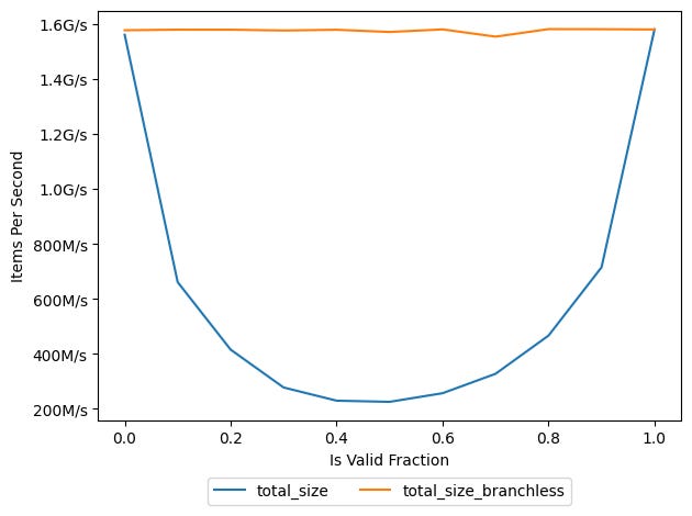
To confirm this, we can look at perf stat again, and see that even with a 0.5 fraction, we have a very small number of mispredicted branches.

While we’ve drastically improved our performance and made the performance relatively independent of the input, we can go further by improving how we execute this branchless code. Multiplication is a relatively expensive operation. Looking at the timeline view in LLVM-MCA of a simple multiply of two 64 bit integers, we see it takes an estimated 3 cycles to execute. Other operations, specifically the bitwise-and operation can be executed within a single cycle. As such, if we can replace our multiplication with a bitwise-and, we likely stand to improve our performance in this branchless case.

In order to achieve this, we want to mask our value with all 1s in the case where is_valid returns true, and mask with all 0s in the case where is_valid returns false. To do this, we’ll store our masks in a 2 element array, indexed by is_valid. So index=0 (is_valid is false) stores 0u, while index=1 (is_valid is true) stores 0xFFFFF... Using two’s complement, the representation of -1 is all 1 bits which we can use that to build our stored value. As such we have the following

When we now include that in our benchmark, we see that we’ve improved on our multiplication by a factor of about 18%, reaching over 1.8 billion objects per second!

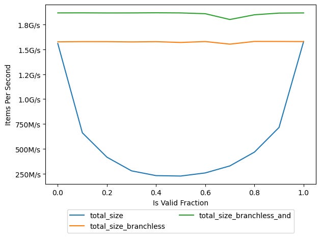
While this may seem that branchless programming is a great tool to start using everywhere, there are some potentially major tradeoffs that need to be considered. First, as we see when our branches are well predicted, there’s little performance difference between the branching and branchless implementations. As such it’s a good idea to measure first with perf before assuming that a branch is actually poorly predicted.

Additionally, in our case one of the reasons the performance gain was so much higher is because the branch was poorly predicted and the work to run our get_size function was so minimal. In this setup, the get_size was able to be inlined by the compiler, making the call to it extremely cheap. If we instead forced the compiler to not inline the function with __attribute__((__noinline__)) we get a different measurement of performance.

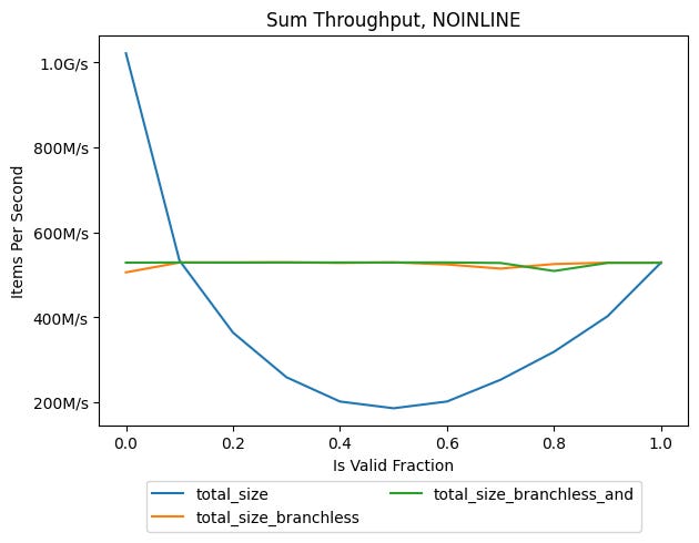
Now we see our branchless implementations are significantly underperforming when the objects are never valid, though still coming out on top when the branch is poorly predicted. To quantify this, we’ll run the benchmark with a configurable padding of nop instructions within the get_size function, and a fixed 0.5 is valid ratio, as follows. This will allow us to simulate making our function more costly to invoke.

As you can see, the compiler optimizes out the for loop, but leaves in the nop instructions thereby padding our function length. When we plot out the throughput as a function of number of nops executed, and a constant 0.5 fraction of is_valid, we get the following results

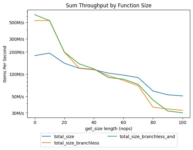
In this log scale graph, we can see when there are less than 30 nops, the performance of the non-inlined branchless implementations still beats out the naive implementation. However as the size of the function increases, the fact that the branchless implementations must execute the get_size function twice as often as the naive implemenation starts to weigh on performance, eventually outweighing the cost of the branch mispredictions.

As we see, there’s a potentially major downside to the branchless implementation as the function to unconditionally call grows in size. One solution to this, depending on the domain, would be to reorganize the data so the branches are easier to predict. In this case, if we were repeatedly going to be processing this data, we could instead sort the vector of objects once, so all the valid objects are at the end, then can be assured that our branch predictor will be very likely to be correct in its guesses since it consistently can learn is_valid as it iterates over the sorted array. The performance for the sorted vector is as follows

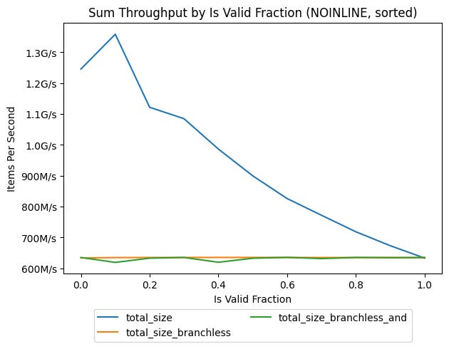
This branch is now fully predictable across all is_valid fractions, and and the throughput in the branch implementation is almost purely a function of how many noinline get_size function calls are made. Our well predicted branch beats or ties the branchless implementations at all is_valid fractions. Of course, now that we know beforehand which part of our vector is valid, we could even rewrite our datastructure in a more data-oriented fashion and eliminate the branch entirely, but that will be discussed in a future post.

Through this post, we’ve demonstrated where branches fit into the CPU instruction stream, how they interrupt the pipelined flow of instructions, and how modern hardware attempts to use branch prediction and speculative execution to mitigate these bubbles in the instruction stream. We were able to improve the performance of our poorly predicted branch by using branchless programming techniques, but also demonstrated how these techniques must be used with care to avoid pessimizing the performance of a system. The source code for this post is available on GitHub.

Hopefully this explanation has been helpful, if you have questions, comments or feedback, please leave them below. Thank you for reading and please subscribe for more software and performance engineering posts!