Updated LP Profitability Data

TL;DR

• An earlier version of this data was included in a paper I posted online, which included several rabbit trails, such as data on pool arbitrageurs and a mechanism to recapture arbitrageur profit to make LPs profitable.

• This version presents only the LP profitability data.

• I added five months of data, but the general results are the same.

Automated market maker (AMM) users and developers widely recognize that restricted-range (v3) liquidity providers (LPs) generate negative net profitability, yet their documentation is weak. AMM revenue, fees, are straightforward to calculate, but the LP’s expense from its negative gamma position, and the relevant active capital within an AMM, is not. The significant literature on AMMs examines various LP strategies and nuances to the standard v3 AMM, but the most fundamental datapoint—a metric of average v3 LP net profitability—is largely hidden, if mentioned at all, in these papers.

In practice, online data providers, including the AMM protocols themselves, present gross LP profits on their dashboards, which are revenues without expenses. This is usually presented as an annual percentage yield (APY) by multiplying the fee revenue over the past n days by 365/n, then dividing by the total value locked (TVL) in the pool. Worse still, these LP APYs often include rewards from minting protocol tokens used to jump-start initial adoption. Printing tokens and giving them to LPs effectively transfers wealth from existing token holders to the LPs and does not reflect the LPs’ fundamental profitability; instead, it reflects the popularity of marketing programs in crypto. LPs have become accustomed to seeing LP APYs well above 50% across most pools, yet still losing money after expenses.

This post demonstrates that the LP expense metric—gamma expense relative to fee revenue—is easy to calculate and enables comparisons across pools. The stationary variable cost ratio applies to any holding duration and has the same interpretation, whether the numeraire token is ETH or a stablecoin. Using data on 24 pools over the past five years, I document that v2 LPs make a net profit, while v3 LPs do not, at statistically significant levels; latency and fee tier do not significantly impact this outcome.

Ultimately, users want to know the APYs for their positions, but this is not straightforward because the relative liquidity of an LP position changes throughout the day as prices move into different ranges and LPs add and remove liquidity. Nonetheless, it is feasible to estimate this given an estimate of the expense/revenue ratio. Most importantly, if the expense/revenue ratio is greater than 1.0, the LP collective loses money; if it is less than 1.0, they make a profit. LPs and AMM developers should find a robust LP net profitability metric useful, as a money-losing pool cannot be made profitable through leverage.

I present three different formulas for estimating the LP’s gamma expense, all well-known in the literature. For the v2 pools, the three expense metrics are virtually identical. For v3 pools, they are consistent and highly correlated. Still, I find the ‘markout IL’ optimal due to its simplicity, and it avoids problems created by the correlation between pool liquidity and price movements. LP profitability is then compared for various types of pools. In general, v2 LPs generate positive net profits, while v3 LPs lose money regardless of latency or fee.

Data comes from 24 pools across four chains: Ethereum main net, Arbitrum, Base, and Avalanche C-chain. These are all Uniswap pools except for two TraderJoe pools. Data are pulled from swap log events, which, for v3 trades, provide the end-of-trade pool price and liquidity. For v2 swaps, this liquidity and end-of-trade price are derived from the ‘sync’ event log generated at the time of the trade. However, given v2 liquidity does not change significantly intraday, one can use token and price changes within a day to get a reasonable estimate of v2 liquidity without having to pull the sync event log data.

Many note that IL and LP gamma expenses differ, but the similarities are much more profound. IL refers to a specific start and end time, generating a datapoint, while the gamma expense refers to a rate multiplied by a time. It is like the difference between a squared return and a variance estimate, which is calculated from squared returns. The expected IL and gamma expense are identical.

I initially used three metrics that differ in their inputs.

This formula uses only the token amounts in swap event logs and the end-of-day price. For pools without USD, one uses the token that serves as the numeraire in the price (for most non-stablecoin pools, this is typically ETH). For liquid pools, using the last trade price as the end-of-day price is as effective as using a CEX price, as the AMM price will generally be within the fee of the CEX price, and whether this is near the +fee or -fee price point is random, small, and cancels out over time.

This metric uses a single liquidity estimate and end-of-day prices.

If we apply this to daily data, using the squared log return for that day as variance, we get the price-liquidity metric to three decimal places. One may find this more informative by analyzing a day with considerable intraday volatility that is obscured by the daily return, and estimate a variance using 5-minute returns (e.g., Oct 10, 2025). However, one could also apply the prior two metrics (markout and price-liquidity) at higher frequencies (eg, hourly). In general, people want to estimate LP returns over weeks or months, and in that case, it is used primarily for its simplicity, given monthly liquidity and variance estimates.

The ETH-USDC v2 and v3 pools are the largest and oldest Uniswap pools, making them ideal for examining the robustness of the gamma expense estimates. The gamma expense/fee ratio estimates for the v2 pool are virtually identical, as expected, since v2 pool liquidity changes little. For the v3 pool, the markout price-liquidity estimates are very similar when averaged over a few months.

LP Gamma/Fee Ratio for ETH-USDC v2 and v3 pools

Sample used identical June 2021-Oct 2025 monthly estimates to generate the averages and standard deviations.

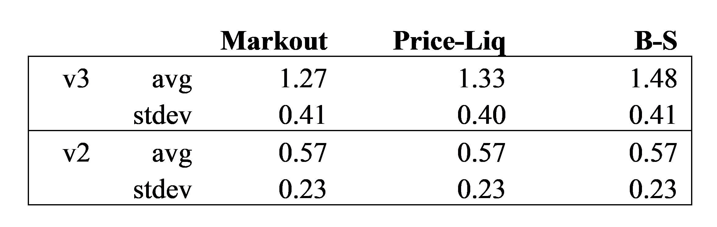
Note: the v3 pool is the ETH-USDC v3 5bp Uniswap mainnet pool; v2 is the ETH-USDC v2 30 bp Uniswap mainnet pool.

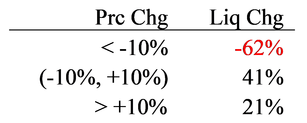
The Black-Scholes ‘variance’ estimate is 10% greater than the markout method due to correlations between liquidity and price changes. Specifically, over a few weeks, a significant price decline generates a liquidity decline significantly greater than the liquidity increase when the price rises. Given that variance is correlated with this tail event, the average liquidity over a month will overstate the actual liquidity in the presence of that large price decline. Significant price declines are correlated with volatility, so an average variance multiplied by average liquidity overestimates the monthly gamma expense.

ETH Price and v3 ETH-USDC 5 bp Liquidity Correlation

Sample used identical daily data from June 2021-Oct 2025 to generate 15-day log returns for price and liquidity. Given that the data were in various price change groups, the average liquidity change was calculated.

The results below are substantively identical regardless of which gamma expense estimator is used. For simplicity, I will use the markout gamma expense estimator below.

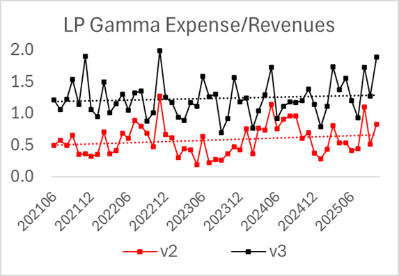
Monthly volatility in the gamma/revenue ratio is significant, suggesting several months of data are needed to obtain a robust estimate. The general pattern of v2 ratios below 1.0 and v3 pool ratios above 1.0 is relatively consistent. The trend is upward, though slightly.

Monthly Gamma/Revenue for ETH-USDC v2 and v3 Pools

IL and Fee data were estimated daily, then used to create monthly averages, and subsequently, a moving average of the monthly averages was calculated.

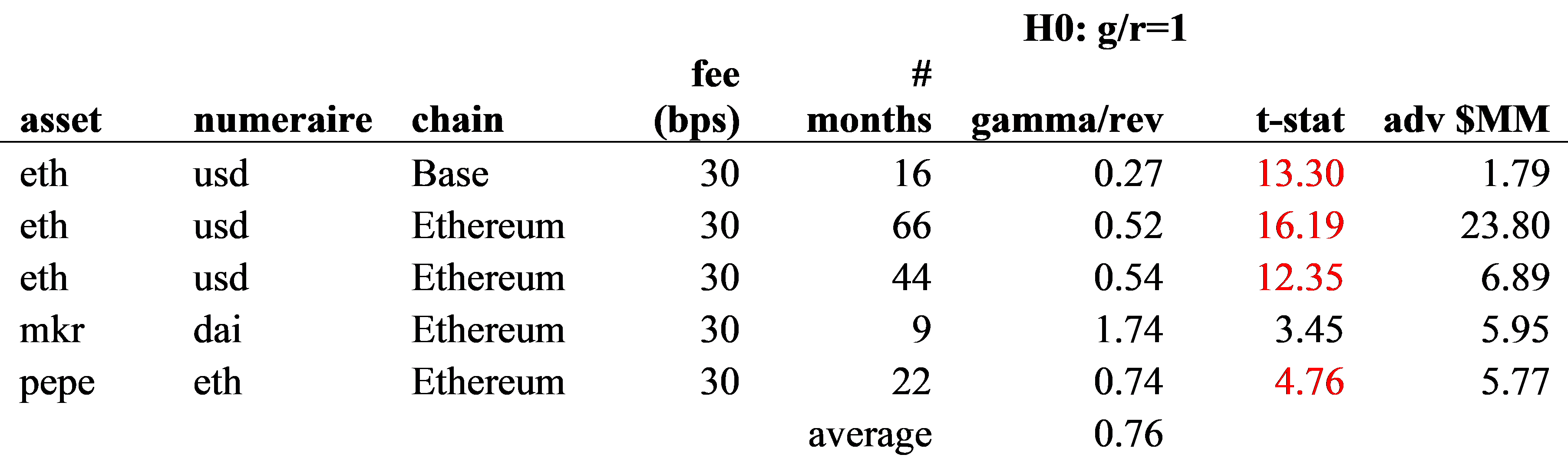
The gamma/fee ratio is significantly below 1.0 for four of the five v2 pools. The only exception is the Maker-Dai v2 pool, which incurred significant LP losses during its brief existence and was terminated in 2024. Aggregating monthly gamma expenses and fees for the v2 and v3 pools using an ADV weighting, the unprofitability of v3 LPs and the profitability of v2 LPs are highly significant.

V2 Lifetime Average Monthly IL/fees by Pool

The t-stat is for the two-tailed test that the gamma/revenue ratio equals 1.0

Of the 18 v3 pools, 13 show statistically significant IL/fee ratios greater than 1.0, indicating the LPs lose money. Three of the five remaining pools generate a statistically significant LP profit, though these are the smallest pools in the sample. The profitable v2 pools are considerably smaller than the v3 pools.

V3 Lifetime Average Monthly IL/fees by Pool

The t-stat is a two-tailed test of whether the gamma expense-to-revenue ratio equals 1.0.

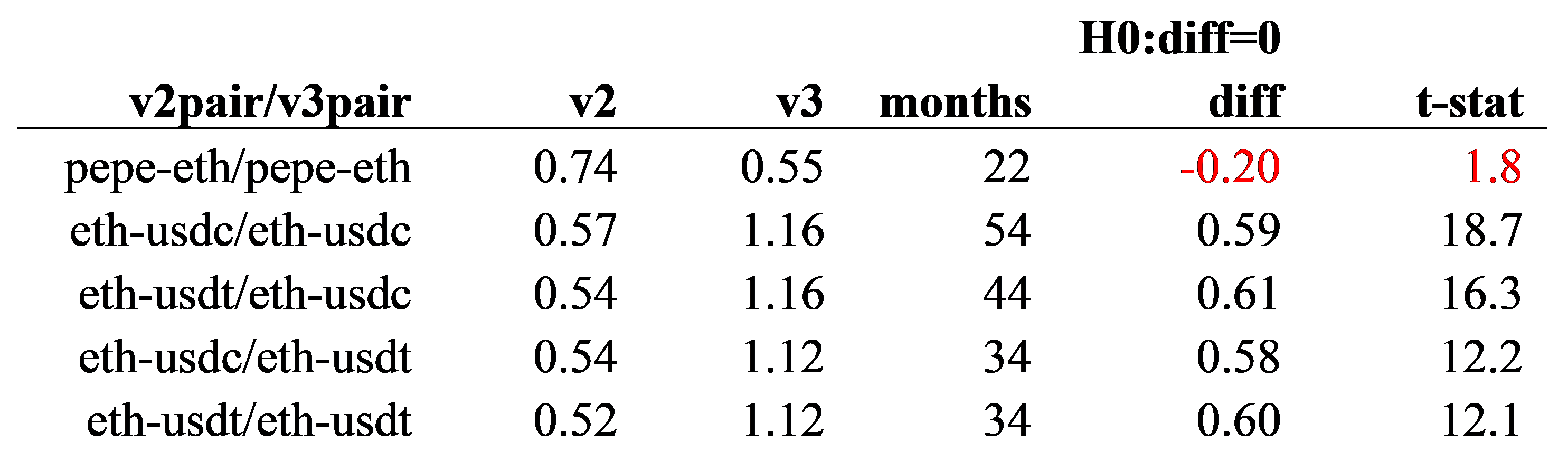
A direct comparison of v2 and v3 LP performance compares pools with identical token pairs and fees, all on the Ethereum mainnet. This uses the intersection of their monthly data, excluding months when either pool is not active, thereby removing noise from months when one pool might have benefited from a low-volatility period, etc. There are four ETH-USD pools: two using USDC and two using USDT, with 30 bp fees for v2 and v3 pools. USDT and USDC are almost perfect substitutes, making comparisons appropriate. For all five comparisons, the v2 LP expense/fee ratio is statistically lower than the v3 LP profitability; thus, v2 LPs generate greater profits than v3 LPs. The v2 pools are all smaller than the v3 pools.

Token Pairs that trade with identical 30 bp fees on Ethereum Mainnet

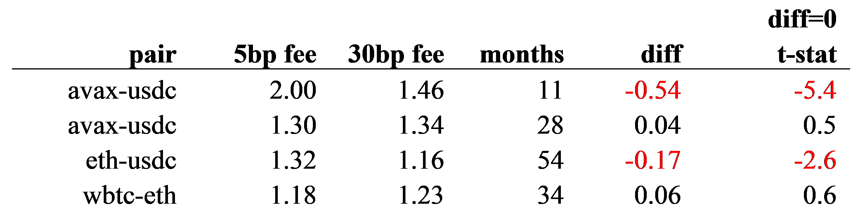
Using identical v3 pools with the same token pairs on the same chain, the higher-fee pools show weak PnL dominance, with the ETH-USD pool showing a statistically significant difference. The Avalanche pools use two TraderJoe pools: the original AVAX-USDC pool with a 20 bp base fee, Uniswap’s AVAX-USDC with a 5 bp base fee, and TraderJoe’s more recent 4 bp fee pool. TraderJoe’s fees vary by asset volatility, but in practice, this adjustment adds just 2 bps to their average fee. The Trader Joe 22 bp fee is the high-fee alternative in both comparisons.

Token pools with the same token pair on v3 but different fees

The first avax-usdc pool compares TraderJoe against TraderJoe, the second Uniswap vs. TraderJoe, all on the Avalanche chain.

A prominent prediction was that lower latency would lead to better LP performance. Using v3 pools with identical token pairs and fees, we see an ambiguous pattern. On two of the four pools, the faster chain has a lower IL/fee ratio, and none of the differences are statistically significant. All LPs in these pools lose money.

V3 pools with the identical token pairs and fees trading on different blockchains

All pools charge 5 bps.

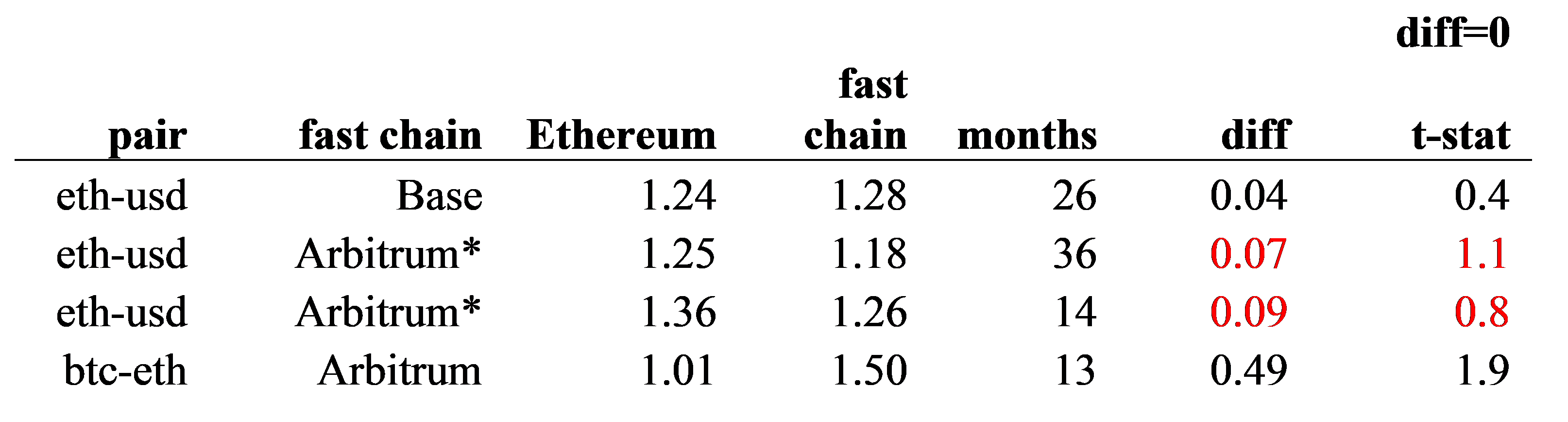
* In the second row, the Arbitrum comp uses USDC, while in the third, it uses USDT.

The IL/fee ratio is a meaningful measure of LP profitability that can be applied across v2 and v3 pools. The variable nature of v3 LP leverage within a pool makes any APY arbitrary. However, given that v2 LP costs are consistently lower than their fees, it is helpful to see what this implies for the more intuitive APY. Initially, net APYs were attractive, though not close to the 40%+ APYs one regularly sees on the web.

Over the past four years, these profitable LP positions have generated APYs of 5-9%, which appear to be reasonable returns for a passive investment on the blockchain. The v2 ETH-USDC pool on Base made an outstanding APY initially, 51%, and while down to 15% in October, it’s still very good. The v2 return of 4-5% seems like a natural equilibrium return for passive capital.

LP Net APY on v2 Pools

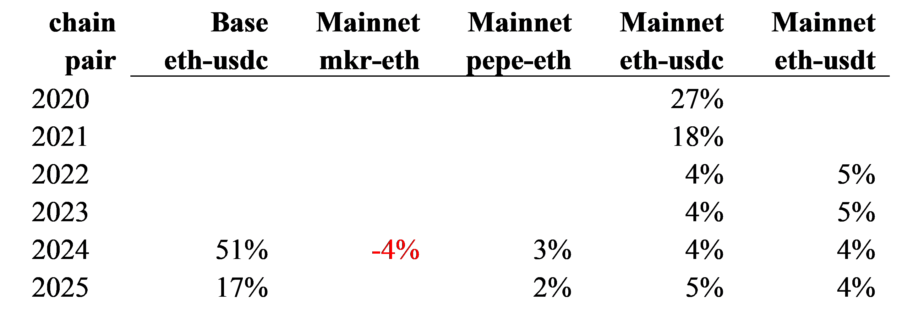
LP Gross APY on v2 Pools

Maximal extractable value (MEV) transactions are often mentioned as hurting LPs, though they primarily affect traders. For example, when a large trade comes in and someone front-runs a retail trade, that retail trader gets a worse fill price. When the arbitrageur reverses the retail trade, this hurts no one and adds volume and thus fees to the LPs. This adds momentary noise to the AMM price and does not affect the standard LPs any AMM designer is targeting. This is because most LPs invest for at least 1 day, and the IL is affected only by the initial and final prices. These trades wash out within a few blocks, leaving no trace on the AMM price.

However, some LPs post liquidity 100 or 1000 times the current liquidity to capture virtually all of a trade, and its fees, paying sequencers to place their liquidity changes just before and after the targeted trade. In this case, fee revenue is reduced by these snipers, as MEV liquidity providers effectively steal LP fees. The chart below shows the liquidity for each transaction on February 24, 2025, for the 5bp USDC-ETH pool, which had 10,000 transactions. There are 137 swaps in which the liquidity was 100 times greater than that of the swaps immediately before and after.

JIT Trade Intraday Pattern

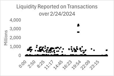
These data are from the ETH-USDC 5bp v3 mainnet Uniswap pool. The median liquidity on this day was around 10 million, so the dots around 1000 each represent a 100-fold temporary increase in liquidity.

These extreme observations reflect ‘just-in-time’(JIT) liquidity, which adds and removes capital within a narrow band, typically 10 basis points wide. This dramatically affects the mean liquidity, which is why median liquidity works better than mean liquidity when estimating gamma expense. Theoretically, they should be excluded because these MEV LPs are not ‘real’ LPs, or at least, not LPs that an AMM designer should target.

Removing these trades from a dataset is difficult, and any mechanism will generate type 1 and type 2 errors. For example, a trade that sees a 100-fold increase in liquidity just before and after the trade would be an MEV trade. However, the extreme liquidity can persist for several blocks, if not minutes. Some liquidity increases are only 5- or 10-fold. There will always be borderline cases that get incorrectly excluded or included.

Fortunately, these trades do not materially affect any of the results generated above. My base dataset used to generate the above results applies MEV exclusion criteria. If I do not remove these trades, the net profitability results do not change significantly. Many pools are unaffected, but for some, this reduces their volume by 5%.

LP gamma/Revenue Including and Excluding JIT Liquidity

This only presents v3 pools because JIT liquidity does not affect v2 pools.

Since its inception, the dominant capital-efficient AMM LPs have lost money. Most people are aware of this, but the data on this subject is sparse. This post presents a simple algorithm for calculating the v3 LP profitability metric that is stationary and allows comparison across pools of different sizes. It also shows that restricted-range LPs have generally lost money, while unrestricted-range LPs have generally made modest profits.