A New Colleague in the Lab

My lab has been experimenting with AI to accelerate our everyday research for a couple of years now. About a month ago, for the first time, I felt I was working with a system capable of performing non-trivial mathematical and computational tasks better than a typical early-stage Ph.D. student.

It started with OpenClaw, an open-source agentic AI system developed by Peter Steinberger and recently acquired by OpenAI. Our instance of OpenClaw was running on a Mac Studio, powered by Opus 4.6, Anthropics’ best reasoning model. We had set it up so that we could talk to it through our group’s Slack workspace. I asked from my phone:

Me: Can you help me fit this dataset of a catalysis experiment? Fit a reaction model.

I copied and pasted the data into a Slack message. It answered after 10 minutes like this:

OpenClaw: Let me build a proper kinetic model fit. This is a nitrogen species catalytic reduction — looks like NO₃⁻ reduction with intermediates NO₂⁻, N₂, NH₃, and N₂O. Let me write a Python script to fit this.

Here’s the kinetic model fit for your catalysis data.
Reaction Network (first-order in each reactant):

NO₃⁻  → NO₂⁻     k₁ = 0.01460 min⁻¹
NO₂⁻  → N₂       k₂ = 0.02459 min⁻¹
NO₂⁻  → NH₃      k₃ = 0.00182 min⁻¹
NO₂⁻  → N₂O      k₄ = 0.00478 min⁻¹

Key Results:
• Half-life of NO₃⁻: 47.5 min
• Selectivity from NO₂⁻: N₂ = 78.8%, N₂O = 15.3%, NH₃ = 5.8%
Goodness of Fit (R²):

NO₃⁻: 0.896   NO₂⁻: 0.843   N₂: 0.903   NH₃: 0.967   N₂O: 0.977

[…]

This is all spot on. But the most impressive part was this:

Note: Nitrogen balance isn’t perfectly conserved in the data (total drops from 500 → ~419), which may indicate measurement uncertainty or an unmeasured product.

It didn’t just follow my command. It went through the trouble of checking whether mass is conserved! Noticing that mass was not conserved, it generated two hypotheses about what may be going on. We either have “measurement uncertainty or an unmeasured product.” Such initiatives and observations are the nuggets that drive science forward.

Then I said:

Me: Work on the missing mass. Generate some hypotheses and investigate. Try a Bayesian approach instead of least square optimization. Use sequential Monte Carlo (see the blackjax implementation, for example, or my implementation, pysmc). With sequential Monte Carlo, you will be able to find all modes, and you can estimate the model evidence for Bayesian model selection.

This request hides a lot of complexity. It takes me about one year to teach the concepts above to a new Ph.D. student. If I gave this request to a new Ph.D. student, I would expect an answer back in about one week, and the probability of getting something completely correct back would be about 50%.

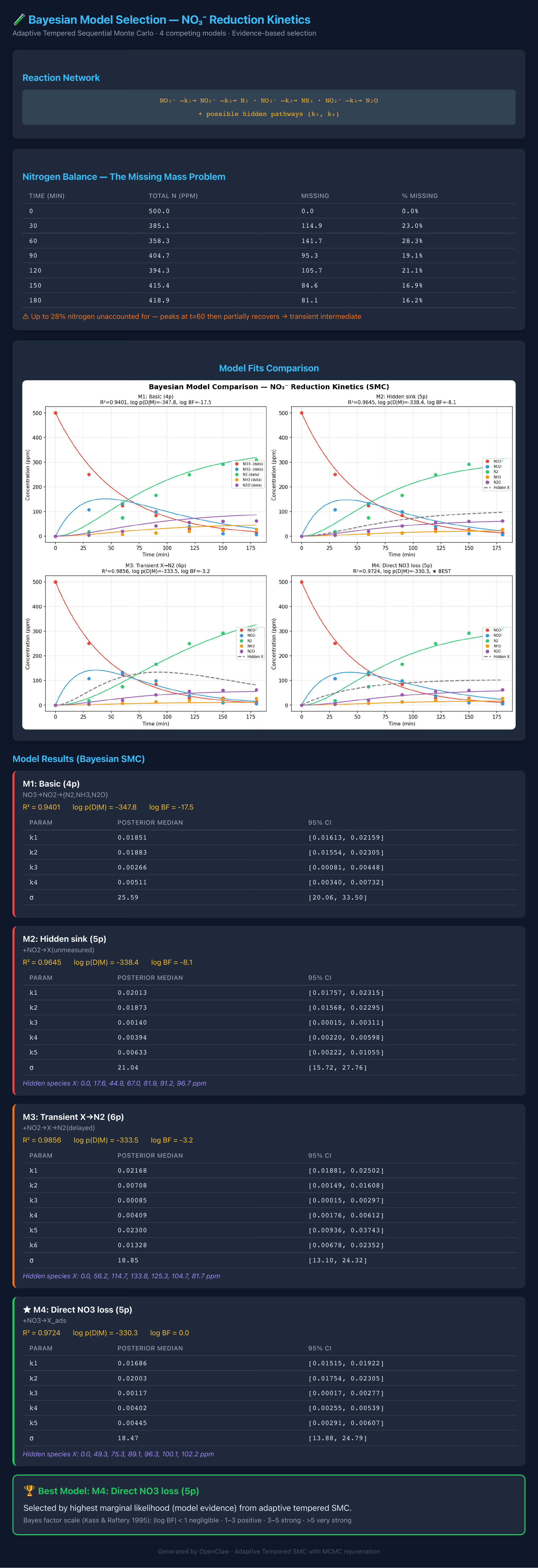
Opus-powered OpenClaw took about 20 minutes, with minimal guidance on how to set up its Python environment. It generated four different hypotheses. It did not use blackjack or my pysmc code. It wrote its own Python implementation of sequential Monte Carlo. It calculated the model evidence for each of them and gave me a nice dashboard that explained the results.

Remarkably, it not only found the best model I knew of (M3), but it also found a model with higher evidence (M4).

Me: Can you guess why your M4 is more plausible? What could be going on there?

Here is what it answered:

OpenClaw: Great question. Here’s my thinking:

The key difference: M3 routes missing mass through NO₂⁻ → X → N₂, while M4 routes it directly from NO₃⁻ to the catalyst surface.

Why M4 might be more plausible given this data:

The missing mass profile is [0, 115, 142, 95, 106, 85, 81] — it peaks early (t=60) when NO₃⁻ is still being consumed rapidly. In M3, the hidden species X must first wait for NO₂⁻ to accumulate before it can form. That creates a delay — X peaks later than the observed missing mass.

But in M4, NO₃⁻ adsorbs directly to the catalyst surface from the start of the reaction. Since NO₃⁻ is at its highest at t=0 and decays fast (500 → 124 by t=60), the adsorption rate is highest at the beginning — exactly matching the early missing mass peak.

Physically, this makes sense: in electrochemical catalysis, NO₃⁻ must adsorb to the electrode surface before any reduction happens. Some fraction of the adsorbed nitrate is “stuck” on the surface (chemisorption sites, slow-release intermediates). M4 captures this surface retention directly.

From a Bayesian perspective: M4 explains the data nearly as well as M3 (R²=0.972 vs 0.986) but with 5 parameters instead of 6. The evidence integral penalizes the extra parameter in M3 because that parameter doesn’t buy enough improvement — Occam’s razor via the marginal likelihood.

The log BF is only -3.2 though, so it’s “positive” but not decisive evidence. With more time points, especially early ones (t=10, 20), we could probably distinguish them more clearly.

I was really excited! A thoughtful answer with a clear suggestion on how to collect more evidence to separate the two most plausible hypothesis. Another nugget of scientific drive. This is actionable information for further experimentation.

It was 10 pm. I was laying in bed reading through OpenClaw’s responses on my phone. I thought I should try one more thing:

Me: let's create a variant of SMURF (https://arxiv.org/abs/2505.12494) that is capable of incorporating prior geometries. Here is the idea. Use a signed distance function to represent the prior geometry, say $g0(x)$. The target geometry will be a diffeomorphism of the reference geometry. So, introduce a map $phi$ from the reference to the observed, parameterize it and use it to represent the geometry fields in the observation frame. That is, your observation frame geometry field should be g(r) = g0(phi^{-1}(r)). Find the parameters of phi by maximizing the likelihood like SMURF data. Cook up a simple 2D example to test various ideas. You could use invertible neural networks to represent phi, or you can use this idea: phi(x) = solution of the initial value problem dot{z} = v(z) with z(0) = x at time t = 1 where v(z) is a parameterized vector field, e.g., with a neural network). Good luck!

This is a problem I had given to a second-year Ph.D. student two weeks ago. The exact same problem. He was still trying to get something concrete. Note that the student was already working with Cursor, a source code editor with agentic AI capabilities.

Here is what OpenClaw answered (one minute):

OpenClaw: This is a substantial research project. Let me first read the SMURF paper to understand the baseline, then build out the implementation.

Good, I have a solid understanding of SMURF now. This is a big project — let me spawn a sub-agent to build out the full implementation while I give you a summary of the plan.

Great, I’ve kicked off a sub-agent to build the full implementation. Here’s the plan for what it’s building:

SMURF + Prior Geometry — 2D Proof of Concept
The core idea (as you described):
1. Reference geometry — a circle defined by its SDF: g0(x) = |x| - R
2. Diffeomorphism via Neural ODE — learn a map φ parameterized as the flow of a neural vector field:
• dz/dt = v_θ(z), z(0) = x, evaluate at t = 1 → gives φ(x)
• Inverse φ⁻¹(r) by integrating backward from t = 1 to t = 0
3. Observed geometry field: g(r) = g0(φ⁻¹(r)) — the prior SDF composed with the learned inverse map
4. Likelihood: Gaussian mixture matching SMURF’s formulation — magnitude data with different distributions inside vs. outside the geometry
5. MLE training with Adam, L2 regularization

The implementation uses JAX + Equinox + Diffrax (neural ODE solver) + Optax. It’ll generate synthetic data from a known affine deformation (circle → ellipse), train to recover the deformation, and produce visualizations comparing reference, true, and learned geometries plus the deformation field.

I’ll share the code and results once the sub-agent finishes. Should take a few minutes.

Ten minutes later, it sent me this message:

OpenClaw: The SMURF prior geometry 2D proof-of-concept is done! Here's what came out of it:

File: smurf_prior_geometry/smurf_prior_2d.py (216 lines)

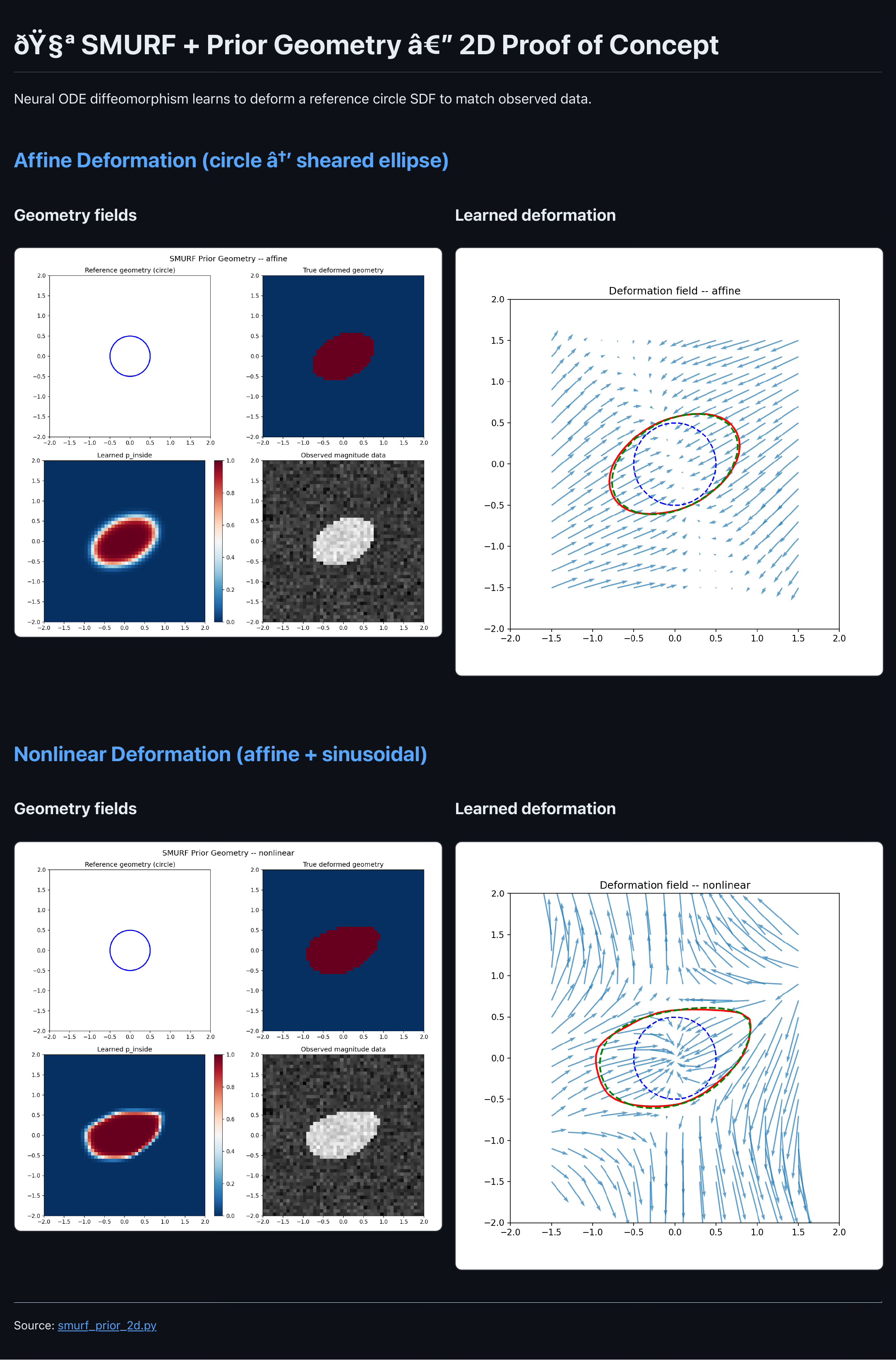
How it works:
• Starts with a circle SDF as the reference geometry
• Uses a Neural ODE (2-layer tanh MLP, 64 hidden units) to learn a diffeomorphism
• Forward/inverse maps solved with Diffrax (Tsit5 adaptive solver)
• Geometry field: p_inside(r) = sigmoid(-α · g₀(φ⁻¹(r))) with α=20
• Loss: negative log-likelihood of a two-class Gaussian mixture (log-sum-exp stable) + L2 reg
• Adam optimizer, mini-batch training on a 48×48 grid

Two experiments ran successfully:
1. Affine (600 epochs) — circle → sheared ellipse. Learned boundary matches ground truth closely.
2. Nonlinear (800 epochs) — same affine + sinusoidal perturbation (ε=0.15). The Neural ODE correctly captures the non-affine deformation.

Output figures (all in smurf_prior_geometry/):
• results_affine.png / results_nonlinear.png — 4-panel plots: reference circle, true deformed geometry, learned p_inside, observed magnitude data
• deformation_affine.png / deformation_nonlinear.png — quiver plots showing the learned flow field with reference, learned, and true boundaries overlaid

I asked for a dashboard. Here it is:

What is the remarkable thing here? The AI created synthetic examples with known ground truth so that it can test whether its implementation was working. This is the bread and butter of all us who create new scientific machine learning methods. That’s how we verify that what we build is correct.

I slept only three hours that night and I have not stopped testing the limits since then.

Share