Wrighting wrongs

I think we usually miss the danger that comes from really smart people. No, it’s not the risk that they can “go to the dark side”—this is usually obvious, and we pretty much deserve what we get if we then continue to follow their lead. In any case, if you just look around you today, you can see that people leading us massively astray don’t even need to be very bright at all. We have other human vulnerabilities that trump intellect pretty much every time.

The real problem with smart people is as follows. Even the brightest make mistakes, and quite because they are bright, they tend to produce magnificent, plausible rationalisations. The danger is that they then truly come to believe their own bullshit! This can be very compelling for us people of lesser intellect. Even similarly bright people are often swept along.

It takes someone different—often even smarter in that specific domain—to call them out, and that refutation is often ignored. Sometimes we need to wait a century for brilliant bullshit to be seen for what it is.1 I have a case in point.

Sir Ronald Aylmer Fisher was brilliant. He excelled as an academic, and some have claimed, perhaps correctly, that he almost singlehandedly built the edifice of modern biostatistics,2 not to mention his other contributions to biology, genetics and mathematics.3 What they often don’t add is that he built biostatistics substantially wrong—an assertion that will no doubt anger many, many smart people who are still in his thrall.

Some of Fisher’s casual, almost throwaway comments were so smart that they kept lesser intellects busy for decades. In my last post, we encountered^⌘ Fisher’s “fundamental theorem of natural selection”. If you read Edwards’ account, Fisher’s wife explained how Fisher thought up this theorem and produced it “at dictation speed” and then just carried on dictating away. It took several decades of misunderstanding and the sad genius of George Price to interpret Fisher’s idea for mere mortals.

It however required the combined smarts of Fisher, Haldane and someone even smarter to come up with population genetics, which is notoriously math-y. It will soon become apparent that Fisher was less than enthusiastic about being called out for misunderstanding important stuff. The consequences were intellectually devastating. We could have advanced 100 years in a bound, but didn’t.

But first, a brief bio of the man who was arguably smarter than Fisher, and usually right: Sewall Wright. We’ll then in turn explore population genetics (while minimising the maths), genetic drift, dominant genes, and after again dumping on Dawkins, we’ll end off with Fisher’s biggest mistake.

There’s a story about Sewall Wright that in his first year of school, he let slip that he knew how to work out cube roots. The catch was that when his teacher called him up to the front of the class to explain, he couldn’t reach the blackboard.4 Apparently, he was then roundly mocked by his peers, which may have produced in him a reflective and somewhat reticent approach.

Years later, after he had somewhat diffidently walked uphill to the summit of academic excellence, he was visited by population geneticist (and later, president of the Genetics Society of America and the American Society of Human Genetics) James F Crow and Newton Morton (one of the founders of genetic epidemiology). Here’s a description of that visit:

“One of his most striking characteristics was his refusal to speculate about anything he had not previously thought through. While Wright was still in Chicago, my then-student Newton Morton and I traveled there to ask him some questions about effective population number. To each question he answered that he didn’t know, and the whole conversation was over in a few minutes. On the way back to Wisconsin, Morton, who neither then nor now was inclined to understate his opinions, said that if this was one of the world’s greatest geneticists the subject was in a sad state. But a few days later, in response to [our] written questions, we got a 14-page, hand-written letter with everything. Every question was answered carefully, with full derivations.” — James F Crow, 1988.

But Wright’s other feature was that after he had worked things out properly, he refused to be intimidated. It also turns out that he was usually right. He had another advantage here—he outlived the opposition.

Wright wrote his first booklet at the age of 7 and just before his untimely death in 1988 at the age of 99 years5 he was fussing about the reprints of the last of his 212 papers. He was a superb and assiduous teacher, collaborator and reviewer. In 1904, at the age of 15, he helped print Carl Sandburg’s first volume of poetry In Reckless Ecstasy on his father’s printing press; after publishing his first paper in 1912, he founded population genetics with Fisher and Haldane; he worked out the importance of genetic drift, inventing F-statistics and the inbreeding coefficient. He also had a remarkable impact on economics—despite being chased away initially because “an animal husbandman had no business writing about economics”. Ah yes! He studied guinea pigs too. We’ll get to that.

Fisher disagreed with him on many things: fitness landscapes, genetic drift, and dominant genes. Mostly, Fisher has turned out to be wrong.6 Let’s however start with their more-or-less collaborative success.

The discipline of population genetics is often attributed to the combined efforts of Fisher, Haldane and Wright. The main theme here is genetic differences within and among populations. The maths is often rather heavy, and not for the timid. Let’s keep it simple.

I’ve previously been a bit rude^⌘ about mathematician GH Hardy’s self-expressed desire not to do maths that was in any way useful, but he nevertheless contributed the concept of a ‘Hardy-Weinberg equilibrium’.7 Let’s say you have a population with several different alleles at a single gene locus. The central idea here is that, shorn of other influences, allele frequencies in a population will not change across the generations.

Because we have two copies of genes at a given locus—let’s call the alleles A and B—we can expect that if the respective frequencies of A and B are p and q, then the respective frequencies of AA, AB and BB are p², 2pq and q². In the picture above, you can see neat graphical representations (‘Punnett squares’).8 of how the numbers work out for three and four alleles. Trim off the r’s and esses for the two-allele case.9

Of course, there are just so many ways that this equilibrium can be upset: not only natural selection but also non-random choice of mates, new mutations, genetic drift, and more. Analysis becomes tricky. Speaking of which here’s a note by Wright on The Distribution of Gene Frequencies in Populations.

The first attempt at a solution was made by Fisher who used a transformation of scale, θ = cos^-1(1 - 2q), designed to give a uniform sampling variance, for all values of q. He attempted to express the conditions in a differential equation but reached erroneous conclusions. My first note on the subject was in 1929, the detailed account appearing in 1931. Fisher (1930) after inspection of the latter paper in manuscript was able to correct his method so as to yield results in agreement in a number of special cases. S Wright, 1937.

The fun starts! You can imagine that Fisher might have just been slightly miffed at being thus corrected in public. And it showed in subsequent interactions. In the following several sections, we’ll discover that simply attributing ‘population genetics’ to the combined work of three geniuses glosses over a lot of differences.

The following quote from the same paper by Wright likely didn’t help, either:

In sufficiently small completely isolated populations, the random divergencies of gene frequencies from their equilibrium values become important, tending to bring about approximate fixation of some random combination of genes which is not likely to be a peak combination. The result is a largely nonadaptive differentiation. In extreme cases there may be the deterioration which characteristically follows excessive inbreeding. Isolation may here be considered the dominating evolutionary factor.

Genetic drift refers to random changes in frequency of an allele in a population. Fixation is where a single gene displaces others. Fisher emphasised that—in his opinion—genetic drift must play a tiny role in evolution. We’ve already seen Wright’s opinion, but it was only in the 1960s that Motoo Kimura brought up the idea that most variation is due to random genetic drift of neutral alleles and that one of these can even reach fixation—his “neutral theory”.10

Kimura’s terse Evolutionary rate at the molecular level, published in Nature in 1968, caused quite a stir. He points out that in mammals, amino-acid substitutions occur at about one per 28 million years, for a chain of 100 amino-acids—but over the whole genome, this means a substitution every two years. That’s waaay more than you’d expect if the main player here is natural selection.11

Kimura’s paper was rapidly followed by similar work from Jack King and Thomas Jukes, and got up the noses of people who had been building a fort around the Modern Synthesis, where natural selection was the potent force, and not to be argued with. We’ve already explored^⌘ how much this is off beam, where we first mentioned Kimura. The question is how to test the competing theories. Arguments are ongoing.12

Wright also came up with several F-statistics that allow sensible comparison of gene frequencies, including across different populations. I’m not going to dwell on human variation too much, because more and more, we’re coming to realise how humans are pretty homogeneous at the genetic level. In addition, most human variation is within population groups. The idea of separate ‘races’ is, well, racist claptrap.

Large-scale examination of data on human polymorphism (using Wright’s F_ST) shows that 87% of variation is within population groups; when you compare populations across continents, just 12% of the remainder is explained, and the tiny remaining 1% results from comparison of populations within continents.13

Another ‘point of difference’ between Fisher and Wright involves something that only seems obvious. As Fisher pointed out in 1928, most mutations in Drosophila fruit flies are recessive, in comparison to the dominant ‘wild type’ of the gene.

As one of the main contributors to the Modern Synthesis, Fisher’s explanation for this was of course natural selection: it powerfully eliminated new, “incomplete dominant” mutations, and took care of the rest through new, mitigating gene mutations that make the bad gene recessive.

Wright disagreed in his remarkably sophisticated paper Physiological and evolutionary theories of dominance. As suggested by the above figure from this 1934 refutation of Fisher, the effects of a single mutation will often be mitigated by a cascade of other effects.14 You can see how this ties into their conflicting views about the potency of natural selection as the one thing to bind all.

This debate went on for decades. You may recall how much importance I’ve previously attached to finding uncomfortable facts that refute our most desired theories. This only happened for Fisher’s theory in 1991, because until then, proponents could always find arguments to wiggle out. The killer is H Allen Orr’s A test of Fisher’s theory of dominance.

Previously we discovered Chlamydomonas (Sex Death and Darwin II^⌘), which is haploid except in times of stress, when sex happens. Orr leveraged this quirk. In haploid organisms, the full impact of a mutation is evident, and Fisherian selection simply can’t happen. He shows that in Chlamydomonas, diploid mutations are recessive, and the distribution of mutations is very similar to those seen in Drosophila. Fisher’s take on dominance is dead!

We have yet to get to arguably Fisher’s greatest impact—and his greatest failure. Before we do though, we need to revisit Dawkins!

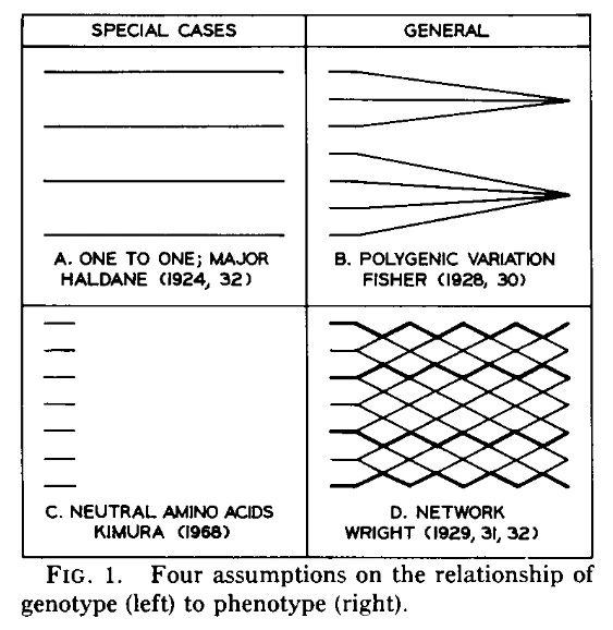
On looking through the list of known human genes (McKusick, 1971), one cannot but be impressed by the number in which the rare allele is responsible for a syndrome that includes multiple effects that are not obviously related. — Sewall Wright, Evolution, 1980

The above graphic is from Wright’s essay Genic and Organismic Selection, a brilliant summary of the state of play up till 1980, and a masterful takedown of Dawkins’ The Selfish Gene. In it, Wright points out something that’s not immediately obvious: in focusing on “the gene’s eye view”, Dawkins is merely aping Fisher, specifically his fundamental theorem. Wright notes that Fisher’s theorem will hold (approximately) for:

“… multifactorial characters in an effectively random-breeding population if the selective differences between the leading alleles of the various loci are constant and all of lower order than the recombination rates of the loci.”

Otherwise, you have trouble. We already understand Kimura’s take in Fig 1C (neutral changes have no phenotypic result, the lines stop). Fig 1A represents a simplistic mosaic of genes. So we’re left with Fig 1B, where genes converge to produce simple phenotypic results, and finally 1D, Wright’s take on things.

He say that he too started off with the simplistic view presented by Fisher (and Dawkins), but then realised he was wrong, based on his study of gene interactions to produce colour, and also based on his extensive experience with inbreeding of animals (which gave rise to his F-coefficient). There are multiple, subtle and unsubtle, non-linear interactions between genes. This is pleiotropy—a single gene can influence a multiplicity of traits, as implied by the quote at the start of this section.

If you read my scathing piece on dire wolves,^⌘ you’ll recall how silly it seems to resurrect an extinct species by “inserting the right genes” into some relative. Wright’s take puts meat on the bones. When an organism ‘adapts’ to changing environmental circumstances, many genes change over time, all interacting subtly with one another. This is usually irreversible. A panda can’t unmake the changes^⌘ that happened to its ancestor’s thumb.

One of Wright’s most powerful metaphors for this pleiotropy and the way it interacts with the complexities of the organism’s environment has been that of an “adaptive landscape”, a low-dimensional metaphor where hills and valleys represent optimal gene combinations in a wildly more complex high-dimensional space. Genes are selected in terms of adaptive topography—if they fit the combination; movement in this space is complex. There’s been a lot of discussion about how appropriate the metaphor is.

And all of this goes head to head with Fisher’s fixation on natural selection as the be-all and end-all, his ideas about dominance, and his rejection of mechanisms like genetic drift! Fisher’s inability to conceive that he might be wrong, and his compensatory behaviour had far bigger consequences, however …

What’s wrong with [null-hypothesis significance testing]15? Well, among many other things, it does not tell us what we want to know, and we so much want to know what we want to know that, out of desperation, we nevertheless believe that it does! —Jacob Cohen, 1990.

If you asked modern statisticians about Fisher’s greatest negative influence, I’m sure that a fair number would plumb for how he stifled Bayesian statistics. P-values, Faugh! In the early 1900s, there was similar enthusiasm for what was then called the ‘method of inverse probability’ and competing methods, but Fisher did a lot to promote his brand, later termed ‘frequentist’.16 Notably, Fisher had a flaming public row with Harold Jeffreys, who tried to resurrect objective Bayesian probability, later picked up by ET Jaynes.^⌘

I will however suggest that Fisher’s influence was more damaging and insidious in another domain. And this is where the guinea pigs come in. Despite his reticence, Wright was known to be unstoppable when he got going on a topic close to his heart. And none was closer than guinea pig genetics. He had access to the breeding records of 40,000 of them. There’s an oft-repeated and endearingly dotty caricature of him lecturing enthusiastically while simultaneously calming an excited guinea pig—and then absentmindedly using the guinea pig to erase the blackboard. He always denied this incident ever happened, of course.

My, he was fond of guinea pigs. He was particularly fond of them because his first, most taxing task as a new researcher at the USDA was to explore the heredity of their coat colour. And it turns out that if you take unselected guinea pigs, 58% of their coat colour is not related to Mendelian genetics!

In his efforts to tease out what was happening, Wright ended up revolutionising not just biology, but statistics and finance too, in how we tease out causal effects. Here’s his fabulous guinea pig graphic:

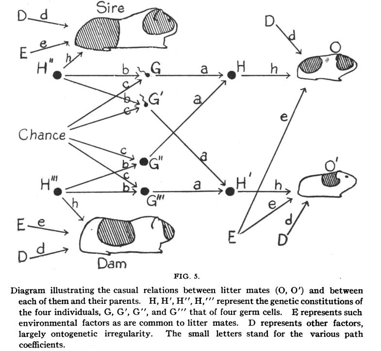
This is from his 1920 paper The relative importance of heredity and environment in determining the piebald pattern of guinea-pigs. Don’t be intimidated by the forest of (causal) arrows, though. Instead, look for the three main influences: hereditary factors (H), common environmental factors (E) such as those experienced by littermates in the womb, and random influences (D).

You can see that this is a Directed Acyclic Graph (DAG), something we’ve looked at before.^⌘ It has however taken us nearly a century to get to that point. Which is a shame, because Wright carefully works through his guinea pig example. He clearly states his assumptions and shows how he does it. The lowercase numbers in his diagram above are path coefficients, and Write points out that these are measures of “the importance of a given path of influence from cause to effect”.

He defines this measure as “the ratio of the variability of the effect to be found when all causes are constant except for the one in question, the variability of which is kept unchanged, to the total variability”, with variability measured by the standard deviation.

He further notes that the squares of the path coefficients measure the degree of determination, and that if the causes are independent, the sum of the squares is 1. He even provides a way to accommodate correlated causes. It’s a pity that he was first attacked, and then ignored—for sixty years.

It’s interesting to contrast the abundantly causal nature of Wright’s writing with Fisher’s approach. Here, I’m going to go with Judea Pearl’s take on things, in his superb The Book of Why.

It’s pretty clear that Fisher didn’t get on with a very large number of people—including Wright, Jerzy Neyman and Jeffreys, but also Egon Pearson, with whom he initially hit it off rather well, until Egon offered some mild criticism that Fisher considered unforgivable. Fisher also squabbled with statistician Arthur Bowley, mathematician Lancelot Hogben, and perhaps most notably epidemiologists Richard Doll and Austin Bradford Hill, who clearly and correctly pointed out that smoking causes lung cancer. Ironically, Fisher, who was a pipe smoker, weaponised “correlation is not causation”. He came up with the bizarre idea that there was some mysterious gene that predisposed to both smoking and lung cancer—and promoted this with funding from tobacco companies. He surely helped kill more than a few people.

The ability to work out causality had been on display for decades. All he needed to do was grasp what Wright was saying. Apart from his dislike of Wright, and his tobacco habit, there was however another factor that hindered his intellect at this specific focus. If you assiduously read my footnote far above on Fisher in 1921 (where he invented modern statistics), you’ll also be aware of some personal enmity between him and Karl Pearson, Egon’s father. Years later, when Fisher was asked to write an obituary for Pearson, his attempts were repeatedly rejected for being too dismissive.

There is therefore a deep irony in Fisher’s acceptance (and, as noted, weaponisation) of a program that was extremely dear to Pearson’s heart. As Pearl points out, early on Pearson started out trying to understand causality and then became massively side-tracked by his discovery of correlation. He then got things arse-about-face, and decided that the important thing was, after all, correlation. And to this day, the best-known correlation coefficient is, of course, Pearson’s.

With his name on the box, Pearson tossed out causation as something peripheral—and subsequent statisticians picked up this obsession with correlation. Statistical discourse explicitly discouraged imputation about causes, with one possible exception. I think Fisher would have agreed with the following quote from Wright:

The ideal method of science is the study of the direct influence of one condition on another in experiments in which all other possible causes of variation are eliminated.” (1921, J Agric Res,20:557)

Fisher’s agricultural plots, where everything was under the control of prospective randomisation. The problem is that life isn’t usually that simple, and you can’t randomise and mechanise everyone and everything. We have seen that Wright has a causal solution: draw an appropriate DAG, work out the coefficients, make a causal inference if you can. Fisher gave us a lasting legacy of none of that.

For now, we’ve finished our brief dip into population genetics and ultimately, the maths of causality. We’ve seen how Sewall Wright’s brilliant insights lay fallow for decades, in a similar way to the neglect of Mendel, and many others who were simply “before their time”. One point of omission is however pretty important. I gave JBS Haldane short shrift. I’ll try to remedy this in my next and penultimate post on evolution, which takes us right back to the beginning. ➵ How on Earth did life originate?

My 2c, Dr Jo.

^{⌘ This symbol is used to indicate posts where I’ve discussed the flagged topic in more detail}