How to be Universal and Natural

If you read many higher-level mathematics texts, you are likely to come across a phrase like “there exists a natural map between [object] and [object].” For instance, in the context of Hilbert spaces or Riemannian geometry, the author may write that there is a natural map between the vector space and its dual.

You might well be forgiven for assuming that the word “natural” here is not meant to have any formal meaning—that it is some vague notion that this is an obvious construction, or it is what is drawn to define. But, actually, “naturality” does have an entirely concrete, mathematical meaning, coming from category theory. That is what we are going to explore today.

I will assume a basic understanding of category theory—i.e., that one is familiar with what a category, the opposite category, a morphism, a functor, and a commutative diagram are. If you aren’t familiar with those, you might look at my earlier post about precisely that.

In this article, our principal aim is to define what a “universal property” is, and give a couple of examples. We’ll then pivot and discuss natural transformations. The reason why I want to cover both here is that they are very important to set up what I would like to talk about next time: adjoint functors. And they share a basic commonality in that they are both two of the most basic, yet non-trivial, category-theoretic constructions.1 And they are both helpful in understanding how category theory captures how we think about “coordinate-free” definitions.

Anyway. Let’s start.

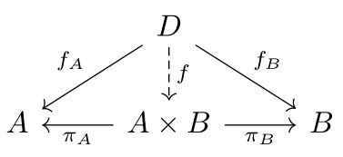
In my earlier article, I gave an intuitive description of what a universal property is: something satisfies a universal property if, for any object, there is always some fixed form of commutative diagram. The example that I gave was for the product A×B of two objects A and B, which is defined by the universal property that for any object D with morphisms f_A: D→A, f_B: D→B, there is a unique morphism f: D→A×B such that the following diagram commutes:

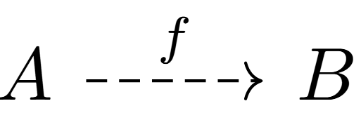
Another—seemingly much more basic—example is that of an initial object. Recall that an object A is initial if for all objects B, there exists a unique morphism f: A→B. In other words, it is defined by the following commutative diagram.

Now, what is the general definition of a universal property? Well, actually one can give a remarkably brief description: an object satisfies a universal property if it is the initial object in some category.

At first glance, this might seem weirdly restrictive—surely this can’t possibly capture all of the variations that we might want to consider… can it? For example, how could one possibly express our definition of A×B in terms of initial objects?

Here’s how. Suppose that we are trying to define the product of objects A, B in a category C. Consider the following category: it has

1. objects that are triples (D, f_A, f_B), where D is an object in C, along with morphisms f_A: D→A and f_B: D→B, and

2. morphisms are just morphisms in C, but with the stipulation that g:(D, f_A, f_B)→(E, f′_A, f′_B) must make the following diagram commute.

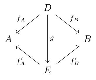
When you unpack the definitions, you realize that actually A×B is precisely the terminal object in this category. Ah! But that means that it is the initial object in the opposite category, and so we are done.2

With a little bit of thought, you’ll see that we can always do something like this—make the objects in your category the “independent” objects in the diagram, along with morphisms to the “dependent” objects, and then make the morphisms be morphisms between such objects that satisfy the desired commutative diagram. This approach has much to recommend it, including the fact that since initial objects are always unique up to isomorphism, you are always guaranteed that anything defined by a universal property will be unique up to the relevant notion of isomorphism.

Let’s look at some examples.

Let’s talk about the tensor product of vector spaces, important in many areas (such as for defining tensors in physics and differential geometry). This is often defined in a slightly tedious, set-theoretic way. We’ll do it using universal properties instead.

So, let’s suppose that you have some field 𝔽 (if you are unfamiliar with how linear algebra works over general fields, pretend that 𝔽=ℝ and all of the vector spaces that we will talk about look like ℝⁿ for some positive integer n—this is sufficient for a first reading), and two vector spaces V and W over that field.

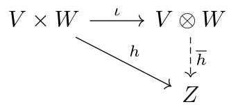
Their tensor product V⊗W is the vector space with a bilinear map ι: V×W→V⊗W satisfying the following universal property: for any vector space Z such that there is a bilinear map h: V×W→Z, there is a unique linear map h̅: V⊗W→Z making the following diagram commutative.

Is this actually a universal property? What is the relevant category? It is the following.

1. Objects are pairs (Z, h), where Z is a vector space over F and h is a bilinear map h: V×W→Z.

2. Morphisms are linear maps ℓ: Z₁→Z₂, with the requirement that if ℓ: (Z₁, h₁)→(Z₂, h₂) is a morphism, then the following diagram is commutative.

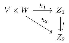
With that definition, V⊗W is indeed the initial object in that category. Therefore, it is unique up to isomorphism—which is to say that any other vector space satisfying this property is related to V⊗W by a bijective linear map.

Furthermore, we can work out from this definition a formal basis for this vector space. Note that, by definition, we have a bilinear map ι: V×W→V⊗W. So, choose a basis {e_i} for V and a basis {f_j} for W. Then V⊗W contains vectors ι(e_i, f_j) for every i, j. Let’s give this a special name: let’s call it e_i⊗f_j.

First, I claim that the vectors e_i⊗f_j span all of V⊗W. To see this, call S the span of these vectors. Then there is clearly a bilinear map defined by what it does to the basis vectors.

Therefore, there must be a corresponding linear map V⊗W→S. This map is clearly surjective. Is it injective? Well, it better be, because if it isn’t, and there is some element α in V⊗W that is not in S, then that element can be sent to any vector in S, and we could still produce a linear map V⊗W→S making the following diagram commutative.

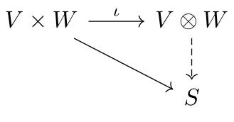
But this breaks uniqueness! So, we must conclude that V⊗W=S, which is to say that V⊗W is generated by vectors e_i⊗f_j, and so its dimension must be dim(V)dim(W).

Despite the fact that we started with an abstract definition, by reasoning through what it says, we eventually recover the concrete description that is more easily phrased in set-theoretic language. But the upside is that:

1. it is now clear that this concrete description has to be the right thing, and

2. we know for a fact that this is describing something uniquely, because it was done via universal property.

In my post on free products of groups, I initially defined the free product of two groups by just sort of concatenating their presentations. I then showed that, actually, the free product satisfies a universal property.

Let me recap. Given two groups G, H, their free product G∗H is the unique (up to isomorphism) group, together with two group homomorphisms ι_G: G→G∗H and ι_H: H→G∗H such that for any group K and any group homomorphisms ϕ: G→K, ψ: H→K, there exists a unique homomorphism ϕ∗ψ: G∗H→K that makes the following diagram commutative.

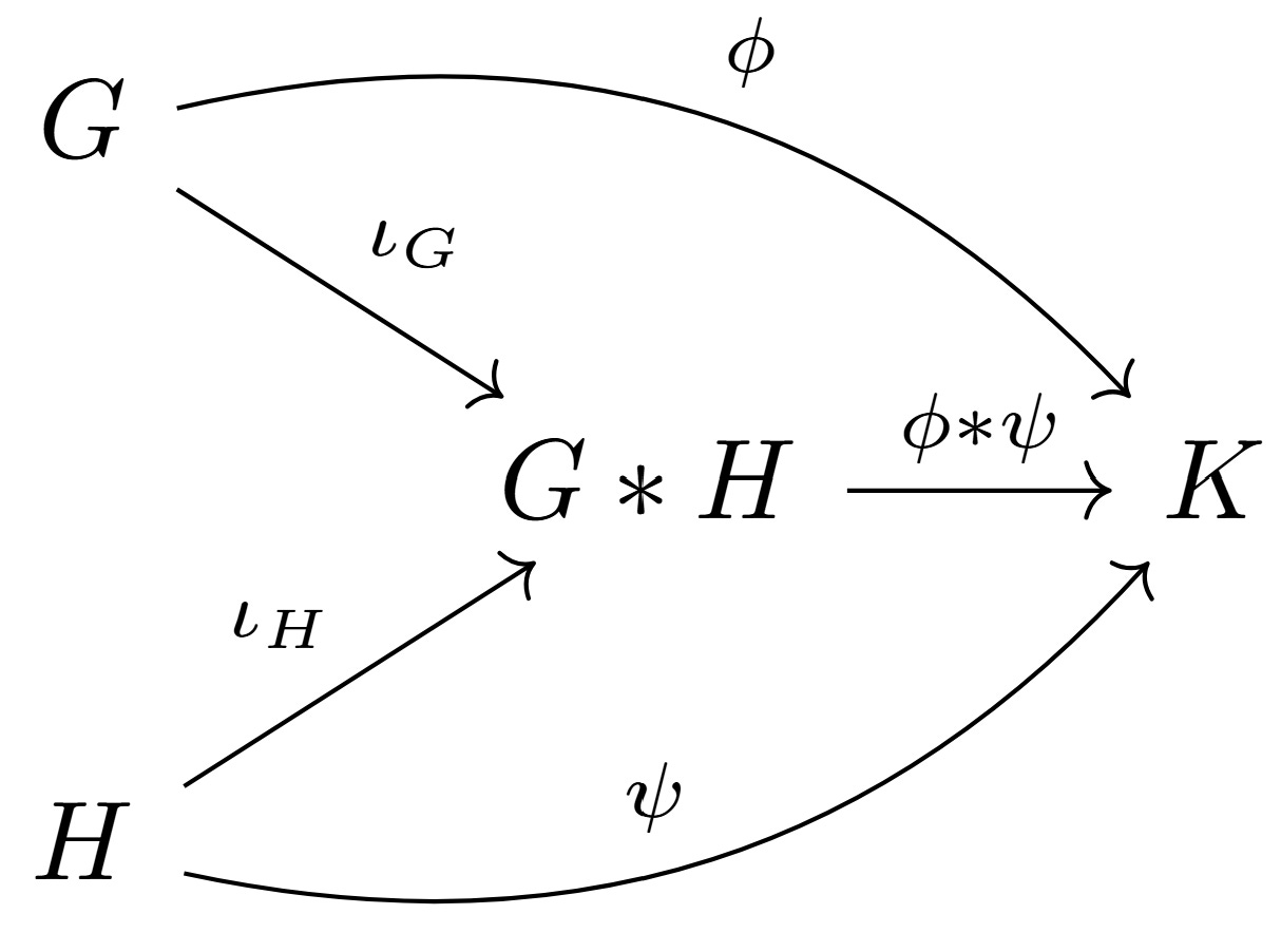
How to see that this is a universal property? Here’s how to build the right category:

1. Objects are triples (ϕ, ψ, K), where ϕ: G→K, ψ: H→K are group homomorphisms.

2. A morphism between two objects (ϕ₁, ψ₁, K₁), (ϕ₂, ψ₂, K₂) is a group homomorphism f: K₁→K₂ such that ϕ₁∘f=ϕ₂∘f.

I leave it to the reader to check that, yes, this is a category, and the free product is the initial object.

Here’s another example of a universal property that will be familiar to those who have studied real analysis. Let X be a metric space. Recall that we say that X is complete if all Cauchy sequences in X converge. A prototypical example that is not complete is ℚ—the collection of rational numbers. This is because, for example, the sequence

does not converge to any rational number, but the terms in the sequence certainly do keep getting closer and closer together. However, it is not so hard to see that if we enlarge the rational numbers a little bit, and, say, throw in √5, then this sequence will converge—specifically, to (√5−1)/2.3 We might therefore posit that we might be able to produce a complete metric space from ℚ by “throwing in” the limits of Cauchy sequences in a systematic way. This is known as the completion of a metric space, and this is actually the standard construction of the real numbers ℝ (which are, precisely, the completion of ℚ).

There are set theoretic ways of constructing the completion of a metric space X, and these are important in that they guarantee that such an object does exist. However, we can give a category theoretic description of the completion as follows: given a metric space X, the completion X̅ is the unique (up to isomorphism) complete metric space together with a uniformly continuous map ι: X→X̅ with the property that for any other complete metric space Y and a uniformly continuous map f: X→Y, there is a unique uniformly continuous map f̅: X̅→Y such that the following diagram commutes.

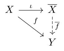
Is this a universal property? Yes, in pretty much the exact same way as the previous example, mutatis mutandis. Specifically, we consider the category of complete metric spaces Y together with uniformly continuous maps f: X→Y, where morphisms are uniformly continuous maps g: Y₁→Y₂ such that the right diagram is commutative.

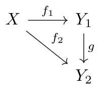
From the universal property, we can prove standard results about the completion. For example, the map ι: X→X̅ is injective. To see this, note that if I have two different points x, y in X, then there exists some uniformly continuous function f: X→[0,1] such that f(x)=0 and f(y)=1.4 This implies that there is a function f̅: X̅→[0,1] such that f̅(ι(t))=f(t). But this implies that f̅(ι(x))=0 and f̅(ι(y))=1, and therefore ι(x)≠ι(y). Since we can do this for any two points x,y, we conclude that ι is injective.

We can also prove that X̅ is the smallest complete metric space containing X. Indeed, choose any complete metric space Y that is a subset of X̅ and contains X. Then there is the obvious inclusion map ι′:X→Y, which must be uniformly continuous, which implies that there is a unique uniformly continuous map ι′: X̅→Y. But on the other hand, clearly there is an inclusion map i: Y→X̅, so we have constructed a map i∘ι’: X̅→X̅. This is troubling, because one checks that this map is uniformly continuous and makes the following diagram commutative.

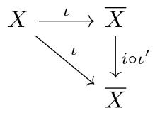
Since the map X̅→X̅ making this diagram commutative is unique (by the universal property), we conclude that i∘ι′=id_X̅. We conclude that the map ι′: X̅→Y is an isomorphism, which is to say that actually Y=X̅. In other words, there is no smaller complete metric space that we could have taken that would have still contained X. Putting everything together, we see that X can be viewed as a dense subset of X̅, which is the way that we usually think of it.

There are more complicated examples that we could give—profinite groups give a fantastic look at why the universal property viewpoint can be so appealing—but let’s put that aside for now and talk about natural transformations. We will motivate them as follows: we have objects in categories, and we have morphisms that define maps between them. We have functors, which define maps between categories. Natural transformations are the next obvious step, as they define maps between functors.

Let’s be specific. Suppose that we are given two categories C and D, and two functors F, G: C→D. A natural transformation η between F and G is a collection of morphisms η_X: F(X)→G(X), one for each object X in C, such that the following diagram is commutative for all morphisms in C.

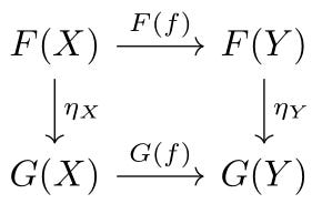
The definition is straightforward enough, but it is likely unclear why we would care very much about natural transformations. The short answer is that natural transformations tell us that there is some sort of “coordinate-free” connection between F and G, which doesn’t depend on any arbitrary choices. To illustrate this, let’s see some examples.

Consider dual vector spaces. Given any field 𝔽 and a vector space V over 𝔽, the dual space V^∗ is defined to be the collection of linear functions λ: V→𝔽. Let’s give a concrete example: take 𝔽=ℝ, and V=ℝ³—i.e., the collection of vectors with three coordinates. Then we can think of V^∗ as the set of 3×1 matrices. An example of an element of V^∗ might be (1, 2, −3), which becomes a linear function returning a real number once we multiply on the left—e.g.

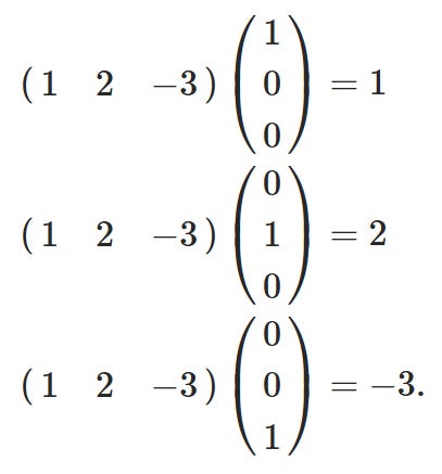
In general, if V is finite-dimensional, there is a bijective linear map (i.e. an isomorphism) V→V^∗. However, there is no one obvious choice for this map. The seemingly clear thing to do is to map

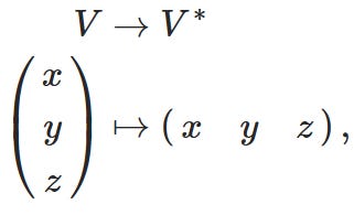
but this is actually a bad choice, because it crucially depends on the particular basis that we select for V. And you never, ever, want your definition to depend on how you choose to represent things.5

On the other hand, consider the double dual V^∗∗, defined precisely how you think it should be: it is the dual space of the dual space of V. I claim that there is a linear map V→V^∗∗ that does not depend on any arbitrary choices, unlike the maps V→V^∗. To wit, consider the following map:

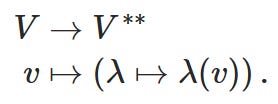
That is, given a vector v in V, we send it to the linear map on V^∗ defined as sending a linear function λ in V^∗ to λ(v). I leave it as an exercise to the reader to check that this really is a linear map, and that it is, in fact, injective (and moreover bijective if V is finite-dimensional). Note that the definition of this map really doesn’t depend on the choice of basis of V, so it looks like it manages to do what we set out to do.

What does this have to do with natural transformations? Quite a lot, actually. This is because we can define a (contravariant) functor ∗:Vec_𝔽→(Vec_𝔽)^op from vector spaces over F to the opposite category of vector spaces over 𝔽, defined as follows:

1. vector spaces V are sent to their duals V^∗, and

2. given a linear map L: V₁→V₂, we send it to the linear map L^∗

   

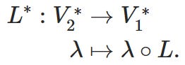
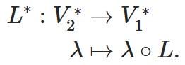
This functor goes to the opposite category rather than Vec_𝔽 itself because it switches the directions of all of the morphisms. However, if we compose this functor with itself twice, then we get a functor ∗∗: Vec_𝔽→Vec_𝔽, which is now an honest-to-goodness functor from the category of vector spaces over 𝔽 to itself. In other words, the double dual is functorial in nature.

This gives us a hint that the observation that there is an injective linear map V→V^∗∗ that is independent of any arbitrary choices can be reinterpreted as a statement about natural transformations. Indeed, here is how: let’s call this map ι_V. Then, given any linear map L: V₁→V₂, the following is a commutative diagram.

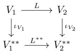
But this is just another way of saying that there is a natural transformation between the double dual functor ∗∗: Vec_𝔽→Vec_𝔽 and the identity functor id: Vec_𝔽→Vec_𝔽 (which just maps every object and morphism back to itself). In particular, if L: V→V is invertible, then all the above diagram is saying is that ι_V=L∘ι_V∘L⁻¹, which is to say that the definition really does not depend on the choice of basis, as claimed.

We usually summarize this relationship by saying that there is a natural map from V to V^∗∗ (if V is finite-dimensional, this map is an isomorphism, and we say that V and V^∗∗ are naturally isomorphic). The way this should be understood is that there is a canonical map V→V^∗∗ for every vector space V, so that together they form a natural transformation.

Have you ever wondered why the trace of a matrix is a meaningful quantity? It is very easy to give a straightforward, computational proof that tr(AB)=tr(BA) for any two square matrices A and B, and from this you can deduce that tr(ABA^-1)=tr(B), which proves that the trace doesn’t depend on your choice of basis. This gives it some apparent worthiness. Later, you learn that it is the sum of the eigenvalues, and this helps reinforce that idea.

But, um, why??? Why is the sum of the entries of one particular diagonal meaningful? Why not the other diagonal? Why not the sum of all the entries in the matrix? The computational proof offers zero insight into this.

Let me give an entirely different proof, which will leverage everything that we have learned so far. In particular, we are going to prove that for vector spaces V, W, there exists a natural map between V^∗⊗W and Hom(V, W)—we’ve defined the former using universal properties and natural maps, and the latter is just the collection of linear maps V→W. Both are, themselves, vector spaces.

First, we need to describe these as functors. We define a category Vec_𝔽^op×Vec_𝔽, with

1. objects (V, W), which are pairs of vector spaces over 𝔽 and

2. morphisms L₁×L₂: V₁×W₁→V₂×W₂, which are the induced maps obtained from linear maps L₁: V₂→V₁, L₂: W₁→W₂ via the universal property of V×W.

Then sending (V, W) to V^∗⊗W or Hom(V, W) will define a functor from this category to Vec_𝔽… once you figure out what to do with the morphisms. Specifically,

1. for V^∗⊗W, we’ll send linear maps L₁×L₂: V₁×W₁→V₂×W₂ to linear maps L₁⊗L₂: V^∗₁⊗W₁→V^∗₂⊗W₂, defined by the universal property of the tensor product;

2. for Hom(V, W), we’ll send linear maps L₁×L₂: V₁×W₁→V₂×W₂ to linear maps

   \(\begin{align*} \text{Hom}(V_1,W_1)&\rightarrow\text{Hom}(V_2,W_2)\\ T&\mapsto L_2 \circ T \circ L_1. \end{align*}\)

Of course, one needs to check that these are functors, but this is straightforward.

Next, we actually need to build the natural transformation between these two functors! We do this in two steps: first, we define a bilinear map V^∗×W→Hom(V, W). Then, we use the universal property of the tensor product to get the desired map.

The bilinear map is fairly simple.

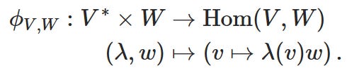
This gives a unique map φ_V,W: V^∗⊗W→Hom(V, W) that makes the following diagram commute.

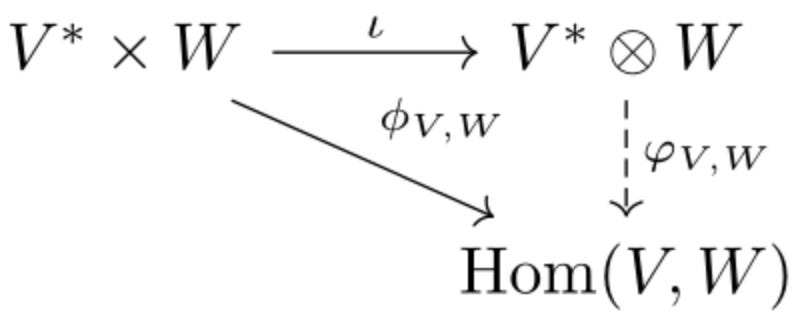
I claim that this unique linear map φ_V,W is precisely the desired natural transformation—that is,

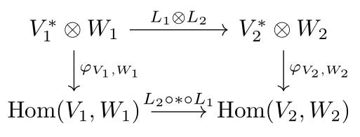
is a commutative diagram for all L₁×L₂: (V₁, W₁)→(V₂, W₂). Let’s actually prove this: we’ll do this by choosing a basis element λ⊗w in V₁^∗⊗W and showing that it ends up in the same place inside Hom(V₂, W₂), regardless of which path we follow. Since this will be true of the basis elements, it must be true of all other vectors by linearity.6

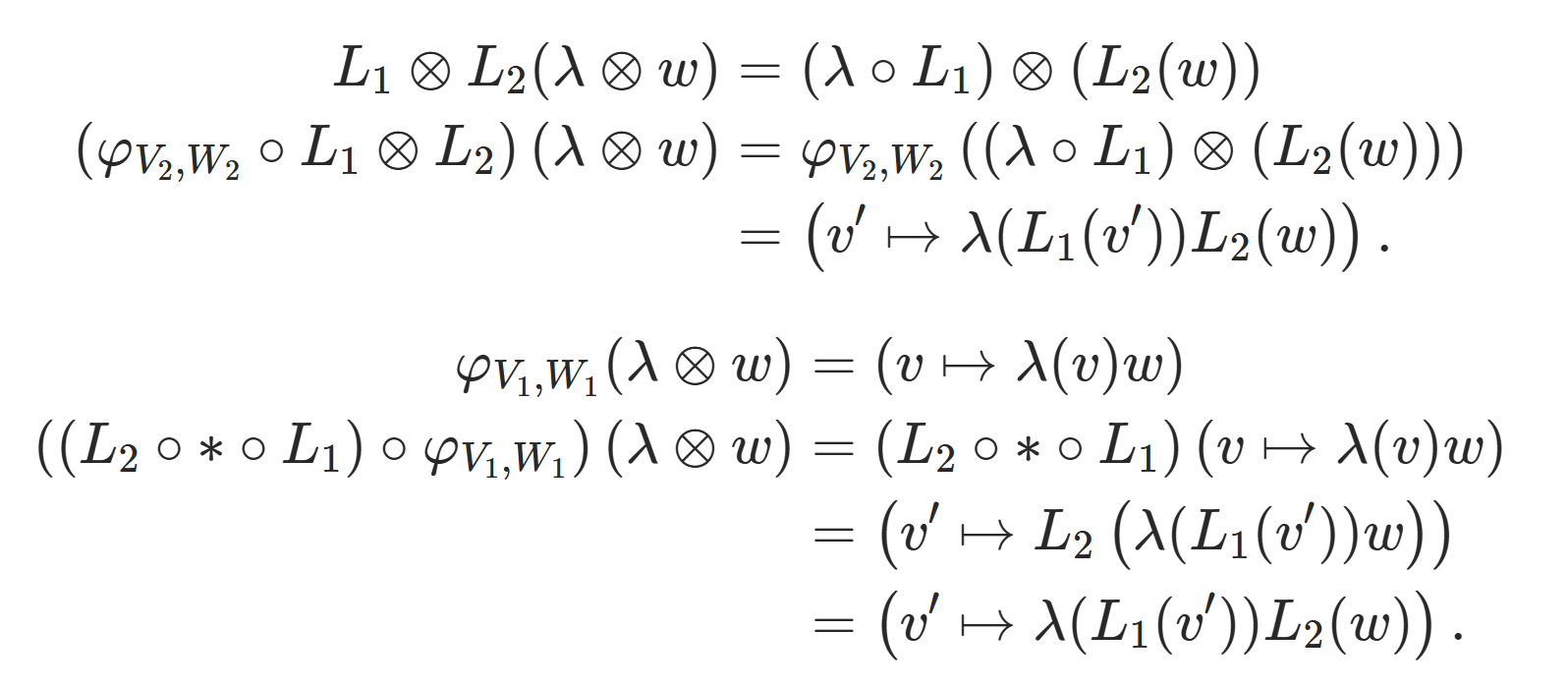
We conclude that, indeed, the diagram is commutative, as claimed. The fact that there is a natural map between V^∗⊗W and Hom(V, W) is quite useful, because it means that all manner of constructions that can be made with one can simply be lifted (functorially) to the other. In particular, when V, W are finite-dimensional, this map is actually an isomorphism. You can see this by counting dimensions on either side: we already worked out that dim(V^∗⊗W)=dim(V^∗)dim(W)=dim(V)dim(W), and of course this is also the dimension of Hom(V, W).

Okay, that was a lot of setup, but we are finally ready to talk about the trace!

What is a square matrix? It is a linear transformation from a vector space back to itself (once you fix a basis). In other words, it is an element of Hom(V, V). However, we know that Hom(V, V) is naturally isomorphic to V^∗⊗V if V is finite-dimensional, so we can equivalently think of it as something in there. The trace then has to be some kind of linear map V^∗⊗V→𝔽.

Hmm. Well, since this is a tensor product, we can start by trying to get a bilinear map V^∗×V→𝔽, and then pushing it to a map V^∗⊗V→𝔽 via the universal property.

But, wait. If you don’t know anything about what this vector space is, there’s really only one thing that you can write down:

Okay. Now, we are going to choose a basis {e_i} for V and see what this map is. Well, the corresponding basis for V^∗⊗V is {e_j^T⊗e_i}, and this map sends e_j^T⊗e_i↦e_j^Te_i—that is, it is 1 if i=j and 0 otherwise. How does this map over Hom(V, V)? Ah, we send e_j^T⊗e_i to the linear transformation that sends v to (e_j^Tv)e_i. What matrix does that correspond to? This is the matrix E_i,j whose coordinates are all 0 except that it as a 1 in the i-th row and j-th column. Every other matrix is a linear combination of these ones. And remember, we send E_i,j to 1 if i=j and 0 otherwise.

Putting everything together, what do we see? This is the trace!

It is immediate from this that the trace doesn’t depend on the choice of basis—our initial definition of the map didn’t make any mention of any basis whatsoever.

Now, you might feel that this is an overcomplicated approach to defining the trace. You might even be right (although I do think that this gives a deeper understanding of what the trace is). But you can do an analogous definition for, say, the determinant (this requires introducing the exterior product), and there I genuinely feel that this gives the cleanest possible definition.