Uncertainty as a Trading Principle

Anyone who has run a machine learning model in a realistic investment pipeline knows that a strategy that looks strong in backtests often loses much of its edge to trading costs, with turnover as the main reason. Models that map firm characteristics directly to portfolio weights are especially exposed, because they rebalance toward a new target every period. The usual response is to penalize turnover: trade less, and give up a little gross return in exchange for lower costs. This helps, but only up to a point, because standard penalties are often blunt. To see why, it helps to ask what the model leaves out when reporting its output.

What it leaves out is any false sense of confidence. A point estimate gives one number for each stock, the weight to hold, with often no indication of how reliable that number is. For forecasting, this could be acceptable. For trading, it is not, because the decision that drives transaction costs is not which positions to hold but whether the positions already held are close enough to their new targets to leave alone. Two stocks can have the same target weight even though the model has estimated one precisely and the other poorly, and a point estimate treats them identically. The information that would distinguish them, how confident the model is in each position, is exactly what it discards.

Return to the turnover penalty. Adding a cost term to the objective does make the model trade less, and it rests on a clean result: penalizing turnover is formally equivalent to placing a prior on the portfolio weights. The problem is that it cannot discriminate. A turnover penalty, like any no-trade band built on a point estimate, treats two positions with the same target weight the same way, regardless of how precisely each is estimated. The point estimate carries no measure of confidence to condition on, so no amount of tuning lets the penalty distinguish a high-confidence position from a marginal one. It lowers the trading bill by treating every position as equally reliable.

A second approach attaches uncertainty to the return forecast, using conformal prediction and related methods that report how confident the model is in its prediction for each stock. This is useful, but it answers a different question. Forecast uncertainty screens which signals to trust before the portfolio is formed; it applies to the inputs of the allocation, not to the allocation itself. It does not address when a position already held is close enough to its target to leave in place. That decision, whether to rebalance or hold, is made at the level of the portfolio weights, and forecast uncertainty does not operate there.

The fix is to attach the uncertainty to the quantity on which the decision depends. Instead of estimating the mapping from characteristics to weights as a single best guess, estimate a distribution over it, so that each weight comes with a credible interval rather than a single value. A Bayesian neural network does this, even for complex portfolio problems. It places a prior over the network’s parameters, the policy that converts characteristics into weights, and the posterior produces, for every stock, a target weight and an interval around it. The width of that interval measures how precisely the model has estimated the position.

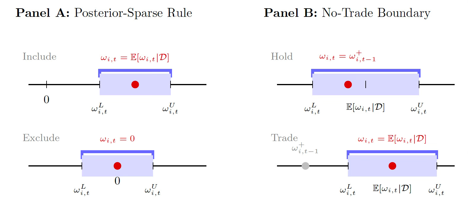
Two trading rules can follow directly from this interval. The first is a no-trade boundary: if the position already held falls inside the credible interval of the new target, leave it, since the difference is within the model’s margin of error. The second is a sparsity rule: drop any position whose interval contains zero, since the model cannot determine the sign of the position. Both come directly from the estimation output. The no-trade boundary is a Bayesian version of the “aim in front of the target” rule from the trading-cost literature, with one important difference: the width of the interval is not an assumption about how quickly signals decay, but a measure of the model’s uncertainty about the position itself.

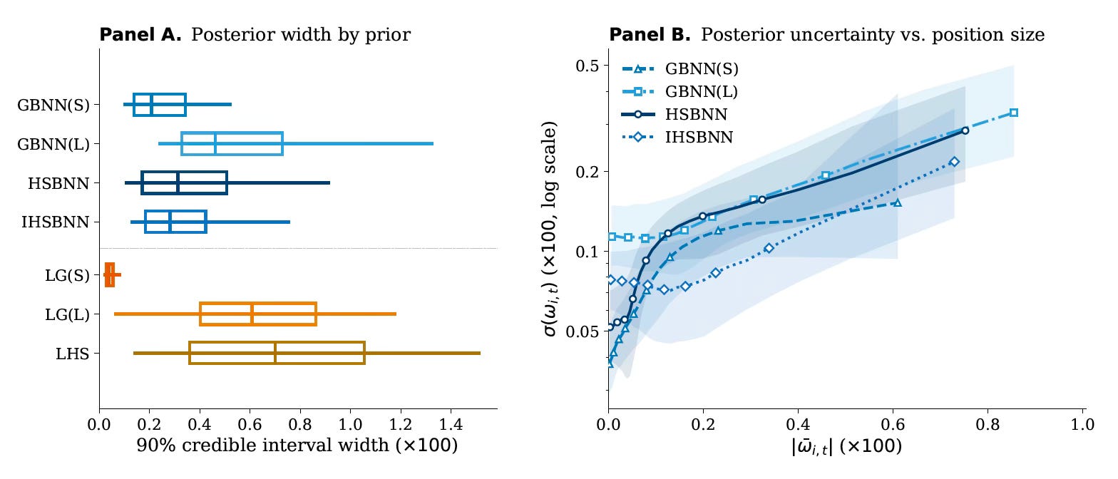
This is the subject of a new paper with my student Xiaoyu Zheng (Queen Mary University of London). What the prior does here is shape the geometry of the uncertainty: how wide the credible interval is on each position, and how that width varies across the portfolio. That geometry determines how much the trading rules save. A sparsity-inducing prior, the horseshoe, produces intervals that are narrow on small positions and wide on large ones. This is a useful pattern because the widest no-trade zones fall on the largest positions, which are the most expensive to trade. A tight, uniform prior produces intervals of roughly equal width across all positions, which leaves the no-trade rule little to act on.

In the data, for U.S. equities with an average of about 4,000 stocks per month, the no-trade boundary reduces turnover by 24 to 45 percent. The margin is large: bid-ask spreads would have to widen fivefold to eightfold before the strategy loses its advantage over the benchmark. The prior also has a practical payoff. The parameter that sets the balance between the model's two objectives has to be chosen, and a horseshoe prior is forgiving about it: set away from its best value, the strategy barely changes. The tight uniform prior is not. Push the balance toward the prior and the portfolio reverts to the benchmark; push it toward the objective, and it trades too much. For an investor who cannot be sure of the right setting, that forgiveness is a real advantage.

One caveat is worth stating directly, as the paper does. The high Sharpe ratios documented come from the breadth of the cross-section, not from any single position being exceptional; restricting the universe to large, liquid NYSE stocks brings them down to more ordinary levels. The advantage of the nonlinear model over a linear one also narrows in that universe, although it persists in statistical and economic terms.

The broader point is that a model’s uncertainty about its own positions has economic value rather than being noise to discard. How confident the model is in a position determines whether that position is worth trading, and the positions not worth trading are where the cost savings come from. On this view, the prior is not only a statistical choice but an economic primitive: placed on the policy parameters rather than the return-generating process, it encodes beliefs about portfolio structure. Even in complex, non-linear, machine learning models.

Based on “Machine Learning Portfolio Choice under Parameter Uncertainty,” joint work with Xiaoyu Zheng (Queen Mary University of London).

Paper available on SSRN: [link]