The Fantastic Promise of quantization

The other day, I noticed that a post from Unsloth, a company we’re friendly with in the space, had gone viral. Specifically, it went viral because they’d managed to quantize GLM-5.2 down to dynamic 1-bit and 2-bit precision while preserving a surprising amount of the original model’s behavior.

Now, to me, this was huge news. The full BF16 version of GLM-5.2 takes up roughly 1.51 TB. Unsloth managed to shrink it to around 217 GB at dynamic 1-bit and 239 GB at dynamic 2-bit. That’s an 86% and 84% reduction in size, respectively.

And the model still works surprisingly well. According to Unsloth’s own results, the dynamic 1-bit version maintained around 76.2% top-1 agreement with the original model, while the dynamic 2-bit version reached roughly 82%. That doesn’t mean the models became 24% or 18% dumber. It means they selected the same top token as the original model that often, which is a much stricter comparison than simply asking whether the final answer was still good. Basically —> they performed uber close to the actual full model.

Lower precision with that much performance left intact? Bro, that’s f**king huge! You can basically shrink an enormous model down to a fraction of its original size and still get pretty good results. And if you managed to survive my memory and inference article, you’ll truly understand why this is so awesome. Smaller models need less memory, fit on fewer pieces of hardware and can be dramatically cheaper to serve.

Transparently, it seemed like a lot of VCs and founders latched onto this point and immediately started jumping for joy. And all that enthusiasm is genuinely awesome. What’s funny, though, is that I think a lot of it exists without a real understanding of what quantization actually is.

So, given my eternal interest in everything LLMs and ML, I’ve taken it upon myself to dive deep into it (your welcome 😁). I’ll get into the math (don’t worry it’s not THAT bad haha), walk through some toy examples and then scale those ideas up to an actual model. From there, I’ll go over some of the ways quantization can turn out badly, prognosticate a bit about how Unsloth pulled this off and finally make a broader claim: effective quantization is going to become a necessity for every single neocloud.

Small Update: After writing all this, I can say that was just super fun to spin up! Hope you enjoy it as much as I did.

Before we can talk about making a model smaller, we need to be clear about what we’re actually shrinking.

An LLM has code that tells the computer how to process tokens, move information through layers and perform an ungodly amount of matrix multiplication. But the code itself isn’t where the model’s learned behavior lives. Most of that is encoded inside the model’s parameters, which are usually called its weights.

A weight is just a number.

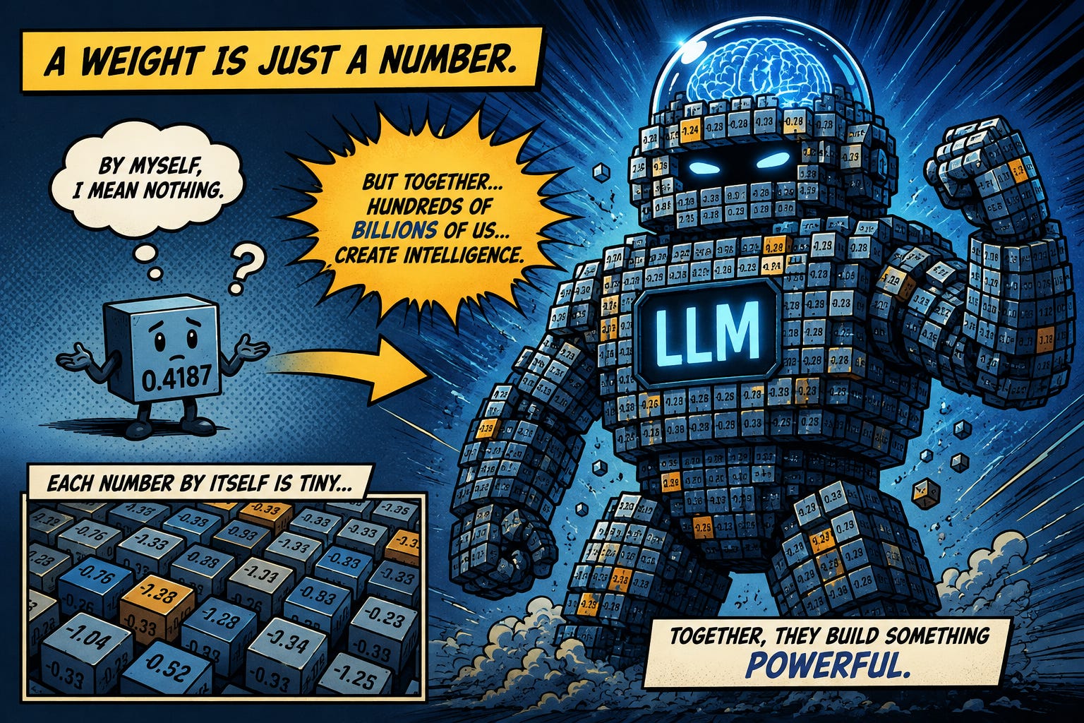
During training, the model sees a gigantic amount of data and repeatedly adjusts these numbers. One weight might move from 0.4187 to 0.4186. Another might move from -1.2041 to -1.2038. Any single change looks completely meaningless. But when you adjust hundreds of billions of weights together, the model slowly gets better at predicting language, writing code and doing all the other slightly spooky things we now expect from it.

The important bit here, no pun intended haha, is that one weight doesn’t usually contain one clean piece of information. There isn’t a specific number inside GLM-5.2 labeled “Paris is the capital of France.” What the model has learned is spread across huge groups of weights and the relationships between them.

Most of those weights are organized into large matrices. When you give the model a prompt, your input gets converted into numbers and repeatedly multiplied through those matrices. The values stored inside them influence what information gets amplified, what gets suppressed and which token the model eventually predicts next.

So when we say that GLM-5.2 contains roughly 754 billion parameters, we’re saying that the model contains roughly 754 billion learned numerical values.

And every one of those values has to be stored somewhere.

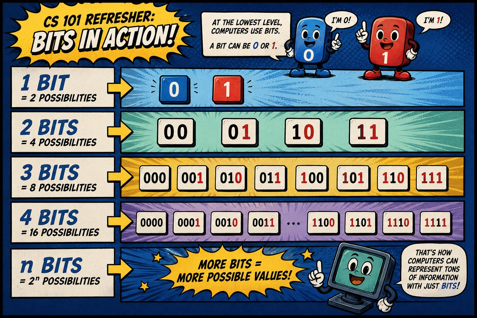
Okay, let’s briefly go back to freshman computer science. For those of you who studied CS and immediately deleted all of this from your brain after the exam, welcome back.

At the lowest level, computers store information using bits. A bit can be in one of two states, which we write as 0 or 1.

One bit gives us two possible patterns:

0
1

Two bits give us four:

00
01
10
11

Three bits give us eight possible patterns, four bits give us 16 and eight bits give us 256. In general, n bits can represent 2ⁿ different patterns.

Those bits are grouped together into bytes:

8 bits = 1 byte
1,000 bytes ≈ 1 kilobyte
1,000 kilobytes ≈ 1 megabyte
1,000 megabytes ≈ 1 gigabyte
1,000 gigabytes ≈ 1 terabyte

There’s some annoying binary-versus-decimal nuance hiding inside those conversions, but we don’t need to ruin everyone’s day with that yet. The important point is that memory and storage are ultimately just enormous collections of bits.

The bit pattern itself also doesn’t tell the computer what it means. The software needs a data format that explains how to interpret it. The same group of bits could represent an integer, part of an image, a letter or a model weight.

LLM weights are commonly stored as floating-point numbers. A format like BF16 uses 16 bits for every value:

1 bit for the sign
8 bits for the exponent
7 bits for the fraction

Those three pieces let BF16 represent positive numbers, negative numbers, very large numbers, very small numbers and values between whole numbers. That range and precision require information, and storing that information takes physical space in memory.

This is the nuance that really matters: a computer doesn’t store the visible characters 0.4187. It stores a 16-bit pattern that the BF16 format interprets as a value close to 0.4187.

And BF16 always uses those same 16 bits. The numbers 0.4187, 0.4 and 12.7 each occupy two bytes if they’re stored as BF16 values. Writing fewer digits on the screen doesn’t save memory. Changing the underlying representation does.

That’s why the storage math works like this:

model weight size ≈ number of parameters × bits per parameter ÷ 8

For GLM-5.2 in BF16:

754 billion parameters × 16 bits ÷ 8
≈ 1.508 trillion bytes
≈ 1.51 TB

Each weight only uses two bytes, which sounds like basically nothing. The problem is that we repeat those two bytes roughly 754 billion times.

Now compare what happens as we use fewer bits:

• BF16 uses 16 bits, or two bytes, per stored value.

• Eight-bit storage uses one byte per value.

• Four-bit storage nominally uses half a byte per value.

• Two-bit storage nominally uses one-quarter of a byte per value.

• One-bit storage nominally uses one-eighth of a byte per value.

You obviously can’t go to a computer store and buy one-quarter of a byte. It works because several tiny values can be packed into a single byte. One byte can hold two 4-bit codes, four 2-bit codes or eight 1-bit codes.

And this is finally where quantization comes in.

At the simplest level, quantization takes weights stored in a format like BF16 and maps them onto a much smaller set of allowed values. Instead of giving every weight its own 16-bit floating-point representation, we store a tiny code that points to a nearby approximation.

We lose some information about each individual weight. But if the approximation is good enough, the model may continue behaving similarly while requiring dramatically less memory.

The number of parameters normally stays the same after quantization. GLM-5.2 doesn’t stop being a roughly 754-billion-parameter model just because Unsloth shrinks it. We aren’t removing most of its weights. We’re representing those same weights with dramatically less data.

That distinction is basically the entire game. Quantization asks how many bits we can take away before the model starts noticeably sucking.

And, as we’re about to see, the answer is apparently quite a lot.

Now that we’ve refreshed the computer science we all conveniently forgot, we can look at what happens when we apply it to GLM-5.2.

The full model contains roughly 754 billion parameters. If each parameter is stored in BF16 using 16 bits, the weights should occupy around 1.51 TB. From there, the theoretical size drops pretty cleanly as we reduce the number of bits per parameter:

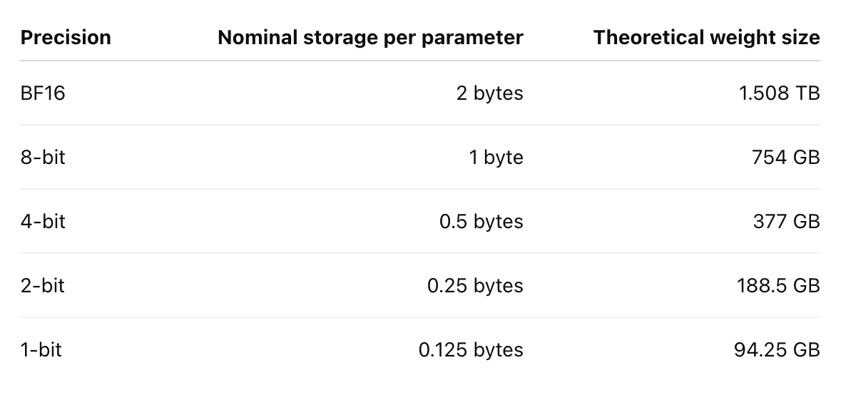
At first glance, the math looks almost suspiciously easy. Cut the bits in half and the model gets cut in half. Keep doing that until your enormous frontier model fits inside something you can buy without first calling NVIDIA and offering them your firstborn child.

But then you look at Unsloth’s actual GLM-5.2 files, and the numbers don’t line up perfectly:

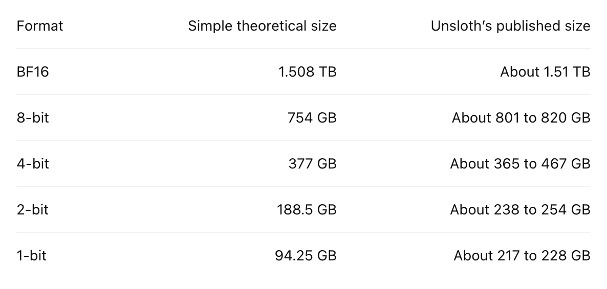
The BF16 number lands almost exactly where we’d expect. But the lower we go, the stranger things get.

The 2-bit version is around 239 GB instead of 188.5 GB. The 1-bit version is around 217 GB instead of 94.25 GB. In fact, dropping from dynamic 2-bit to dynamic 1-bit only saves around 22 GB in the versions we’ve been discussing.

That sounds weird until you understand what the labels actually mean.

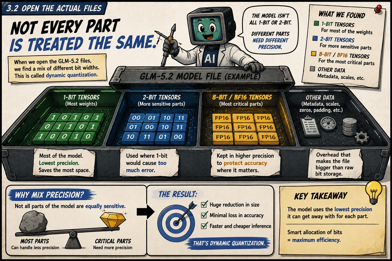
When Unsloth calls something a dynamic 1-bit quant, it doesn’t mean that every single value inside the file has been crushed into exactly one bit. If that were true, GLM-5.2 would land much closer to that theoretical 94 GB number.

Instead, the 1-bit or 2-bit label describes the main quantization approach being applied across much of the model. Some parts remain at higher precision because they’re more sensitive to rounding than others.

We’ll get into the theory behind that later when we talk about quantization error. The short version is that every approximation introduces some error, but errors in certain weights and layers can hurt the model far more than others. Keeping those sensitive areas at higher precision is one of the ways dynamic quantization prevents all those tiny errors from snowballing into complete garbage.

The file also needs to store scales, metadata and other information required to reconstruct and run the low-bit weights. So the final model is really a mixture of precisions rather than 754 billion values all stored in exactly the same format.

A large percentage of the weights might be stored extremely cheaply, while important tensors remain at 4-bit, 8-bit, 16-bit or some other higher precision. Unsloth gets a dramatically smaller model without blindly treating every part of it as equally disposable.

You can even see this in the rough effective storage rate. A 217 GB file spread across 754 billion parameters works out to approximately:

217 billion bytes × 8 ÷ 754 billion parameters
≈ 2.3 bits per parameter

The 239 GB version works out to roughly 2.5 bits per parameter.

Those numbers include the entire file, not just the aggressively quantized weights, so they’re only rough averages. But they make the point pretty clearly: a “dynamic 1-bit” model isn’t literally using one bit for every parameter from beginning to end.

There’s one more nuance here. File size isn’t exactly the same as the memory required to run the model.

The 239 GB quantized file still needs additional memory for things like runtime buffers, temporary calculations and the KV cache. Unsloth estimates around 245 GB of total memory for its dynamic 2-bit version and roughly 223 GB for dynamic 1-bit, although the real requirement will depend on context length and runtime configuration.

Still, the broad result is ridiculous. We started with a model whose BF16 weights occupied roughly 1.51 TB and ended with versions that fit into around a quarter-terabyte of memory.

The model still has roughly 754 billion parameters. We haven’t removed most of its learned numbers. We’ve just become much stingier about how much information we’ll spend representing each one.

The obvious next question is how the hell four little 2-bit codes can stand in for billions of precise floating-point weights without completely destroying the model.

That’s where the actual math begins.

Let’s temporarily forget that GLM-5.2 contains 754 billion parameters. That number is too large to be useful inside anyone’s head.

Instead, imagine that our entire model contains only six weights:

[-1.2, -0.7, -0.1, 0.3, 0.8, 1.4]

Now picture those weights as dots sitting on a number line:

-1.2       -0.7       -0.1    0.3       0.8       1.4
  ●----------●-----------●------●----------●----------●

Each dot represents the numerical value of one weight. The position of the dot matters because that value will eventually be used inside a matrix multiplication.

With BF16, we have 16 bits available for every weight. That gives the computer enough possible bit patterns to place each dot reasonably close to its original position. It can distinguish -0.7 from -0.1, 0.3 from 0.8 and a gigantic number of smaller steps between them.

You can think of BF16 as giving us a very finely marked ruler. It isn’t infinitely precise, but the tick marks are close enough together that every weight can land near the value it’s supposed to represent.

Now we replace those 16 bits with only two.

Two bits give us four possible codes:

00
01
10
11

That means our quantized model only gets four places on the number line.

Not four places between every pair of weights. Four places total for this entire group.

So let’s spread those four available positions across the range covered by our weights:

-1.2              -0.33               0.53               1.4
  ◆-----------------◆-------------------◆------------------◆
 00                01                  10                 11

The diamonds are the only values our 2-bit model is now allowed to use. Every original weight has to move to one of them.

Our -1.2 weight is fine because there’s already a diamond sitting at -1.2. The weight at 1.4 is also fine. Nothing needs to move.

The other four weights aren’t so lucky.

The weight at -0.7 has to slide toward either -1.2 or -0.33. The weight at -0.1 has to pick one of the four available positions too. The same thing happens to 0.3 and 0.8.

You can picture every original dot snapping to the nearest diamond:

Original weight  →  Closest available value
-1.2             →  -1.2
-0.7             →  -0.33
-0.1             →  -0.33
 0.3             →   0.53
 0.8             →   0.53
 1.4             →   1.4

That snapping process is the heart of quantization.

We started with six distinct floating-point values. We ended with four values that the model is allowed to use. Multiple original weights can now collapse onto the same stored value.

The weights at -0.7 and -0.1, for example, both become -0.33. Before quantization, those weights were clearly different. After quantization, the model can no longer tell them apart.

That’s the information we’ve thrown away.

There’s another subtle point here.

The code 01 doesn’t literally mean -0.33. It’s just a two-bit label. We decide that 01 represents approximately -0.33 for this particular group of weights.

In another group, the same code could mean something completely different:

Group A: 01 → -0.33
Group B: 01 → 4.7
Group C: 01 → 0.002

Think of the codes as addresses. The two-bit code tells us which of four available positions to use, but we still need a shared ruler that tells us where those positions sit on the number line.

That ruler is usually described using values such as a scale and sometimes a zero point. We’ll calculate those properly in the next section. For now, just think of them as the information the runtime needs to translate:

01

back into something like:

-0.33

That translation information also takes up memory.

For our tiny six-weight model, this can seem a little silly. The six 2-bit codes use only 12 bits in total, but then we also need to store the ruler explaining what those codes mean. With such a tiny group, the ruler might take up as much space as the weights we saved.

But real models reuse one ruler across a larger group of weights. If 32, 64 or 128 weights share the same scale, the cost of storing that scale gets spread across the entire group.

This is why quantized models aren’t usually exactly as small as the simple bits-per-parameter math suggests. We save a huge amount of space on the weights, but we spend some of it back on scales, metadata and other information needed to interpret them.

There’s also a clean visual way to understand why each weight snaps to a particular diamond.

Imagine drawing a boundary halfway between every pair of available values:

      boundary             boundary             boundary
          |                    |                    |
-1.2      |       -0.33        |        0.53        |       1.4
  ◆-------|---------◆----------|----------◆---------|---------◆

Every original weight to the left of the first boundary maps to 00. Weights between the first and second boundaries map to 01. The next region maps to 10, and the final region maps to 11.

Each diamond effectively owns a section of the number line.

Once a weight falls inside a diamond’s region, we replace it with that diamond’s value. The precise position inside the region is discarded.

That’s why quantization can be understood as placing values into buckets. Every bucket contains a range of original weights, but everything inside that bucket gets reconstructed as the same approximation.

Now draw a little arrow from each original dot to the diamond it snaps toward.

A short arrow means the reconstructed value is close to the original. A long arrow means we’ve changed the weight by a larger amount.

That distance is the quantization error:

quantization error = reconstructed value - original value

For the weight at -0.7:

original value       = -0.7
reconstructed value  = -0.33
error                = -0.33 - (-0.7)
                     = 0.37

The quantized weight is now 0.37 higher than the original.

One error like that probably doesn’t matter. But a real LLM contains billions of weights, and those weights participate in an ungodly number of calculations. If too many important values move too far, the model’s output can begin to drift.

This gives us a much better way to frame the entire problem.

We only have four diamonds. We need to decide where to place them. And we want to place them so that all the original dots have to move as little as possible.

In this first example, we spaced the diamonds evenly across the range. That’s called uniform quantization. It’s simple, intuitive and often useful, but it isn’t always the best choice.

If most of our weights are clustered near zero while one giant outlier sits far away, evenly spacing the diamonds can waste most of our available precision. If certain weights matter far more than others, minimizing the average distance may not protect the calculations we actually care about.

Those are problems we’ll get to later.

For now, we’ve reduced quantization to a picture:

• The dots are the original weights.

• The diamonds are the values we can still represent.

• The boundaries decide which diamond each weight uses.

• The arrows show the error introduced when the dots move.

• The scale is the shared ruler that tells the computer where the diamonds are.

Now we can stop eyeballing the number line and calculate every piece of it ourselves.

At the end of the last section, we had six original weights sitting on a number line and only four diamonds available to represent them.

Our weights were:

[-1.2, -0.7, -0.1, 0.3, 0.8, 1.4]

Because we’re building a 2-bit quantizer, we only have four codes:

00, 01, 10, 11

The question is where those four diamonds should go.

For our first quantizer, we’ll make the simplest reasonable choice. We’ll place one diamond at the smallest weight, one at the largest weight and space the other two evenly between them.

Our smallest weight is -1.2, and our largest is 1.4.

Picture those as the two ends of our ruler:

minimum                                               maximum
 -1.2                                                    1.4
   ◆------------------------------------------------------◆

The total distance between them is:

1.4 - (-1.2) = 2.6

So our weights cover a range of 2.6.

Now we need to fit four diamonds across that range.

This is one of those tiny details that feels obvious after somebody points it out.

Four diamonds don’t create four spaces between them. They create three:

◆--------------◆--------------◆--------------◆
      gap 1           gap 2           gap 3

So we divide the total range by three:

step size = 2.6 ÷ 3
          ≈ 0.8667

This number is usually called the scale. In this simple quantizer, it tells us how far apart our representable values sit on the number line.

Now we can place all four diamonds.

The first one sits at our minimum, -1.2. From there, we repeatedly add the scale:

Code 00:  -1.2
Code 01:  -1.2 + 0.8667
          ≈ -0.3333
Code 10:  -1.2 + 2(0.8667)
          ≈ 0.5333
Code 11:  -1.2 + 3(0.8667)
          = 1.4

Visually, our new 2-bit ruler looks like this:

-1.2              -0.3333              0.5333              1.4
  ◆------------------◆--------------------◆------------------◆
 00                 01                   10                 11

We’ve now built the four values our quantized model is allowed to use.

Let’s start with the original weight 0.8.

It sits between the diamonds at 0.5333 and 1.4:

0.5333             0.8                              1.4
   ◆----------------●--------------------------------◆
  10                                                11

The distance from 0.8 to 0.5333 is approximately:

0.8 - 0.5333 = 0.2667

The distance from 0.8 to 1.4 is:

1.4 - 0.8 = 0.6

So 0.8 is closer to 0.5333. We replace it with code 10.

Original weight:       0.8
Stored code:            10
Reconstructed weight:   0.5333
Quantization error:    -0.2667

The model no longer stores 0.8. It stores the 2-bit code 10, along with the shared information needed to know that 10 represents approximately 0.5333 for this group.

We obviously don’t want to measure every distance by hand. Fortunately, we can calculate the nearest code directly.

For this simple min-max quantizer:

code = round((weight - minimum) ÷ scale)

Let’s plug in our 0.8 weight:

code = round((0.8 - (-1.2)) ÷ 0.8667)
     = round(2.0 ÷ 0.8667)
     = round(2.3076)
     = 2

The integer code 2 is the bit pattern 10.

To turn that code back into an approximate weight, we reverse the process:

reconstructed weight = minimum + (code × scale)

For code 2:

reconstructed weight = -1.2 + (2 × 0.8667)
                     ≈ 0.5333

That pair of equations is our entire toy quantizer:

Quantize:
code = round((weight - minimum) ÷ scale)
Reconstruct:
weight ≈ minimum + (code × scale)

We should also clamp the code between 0 and 3, because those are the only four integers that fit inside two bits. If rounding somehow gives us something outside that range, we push it back to the nearest valid code:

code = clamp(code, 0, 3)

Running every weight through the same process gives us:

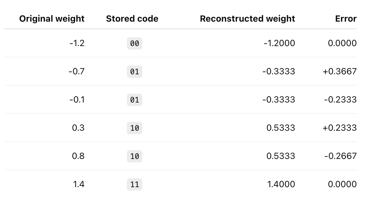
Our original model stored six different numbers:

[-1.2, -0.7, -0.1, 0.3, 0.8, 1.4]

Our 2-bit model stores six tiny codes:

[00, 01, 01, 10, 10, 11]

When those codes are reconstructed, we get:

[-1.2, -0.3333, -0.3333, 0.5333, 0.5333, 1.4]

The first and last weights survived perfectly because we placed diamonds directly on top of them. Everything in the middle moved.

Now we can calculate exactly how much memory all this work saved.

Our original fake model contained six BF16 weights. BF16 uses 16 bits for each value, so the original weights required:

6 weights × 16 bits
= 96 bits

After quantization, each weight is replaced by a 2-bit code:

6 weights × 2 bits
= 12 bits

If we only counted the weight codes, we’d appear to have saved:

96 original bits - 12 quantized bits
= 84 bits saved

That would be an 87.5% reduction:

84 bits saved ÷ 96 original bits
= 87.5%

Or, put another way, the quantized weights alone would be eight times smaller:

96 ÷ 12 = 8

That tracks perfectly with our intuition. Moving from 16 bits per weight to two bits per weight should theoretically give us an eightfold reduction.

But we’re forgetting the ruler.

Our stored codes look like this:

[00, 01, 01, 10, 10, 11]

On their own, those codes don’t tell us that 00 represents -1.2 or that 10 represents approximately 0.5333.

To reconstruct the weights, we also need to store:

• The minimum value: -1.2

• The scale: approximately 0.8667

Those two values describe the ruler used by the entire group:

minimum = -1.2
scale   = 0.8667

Let’s keep the example simple and assume we store both values in BF16. Each one uses 16 bits, so the ruler requires:

2 values × 16 bits
= 32 bits

Our fully loaded quantized representation now looks like this:

12 bits for the six weight codes
+ 32 bits for the shared ruler
= 44 bits total

So we didn’t really shrink the group from 96 bits to 12 bits. We shrank it from 96 bits to 44 bits.

Our actual saving is:

96 original bits - 44 quantized bits
= 52 bits saved

That’s a reduction of roughly:

52 ÷ 96
≈ 54.2%

And the compression ratio is:

96 ÷ 44
≈ 2.18 to 1

That’s still useful, but it’s nowhere near the eightfold reduction we thought we were getting.

The problem is that our group is tiny. We’re storing 32 bits of ruler information to compress only six weights. The ruler represents almost three-quarters of our new storage:

32 ruler bits ÷ 44 total bits
≈ 72.7%

Our 2-bit codes are extremely cheap. The overhead required to interpret them is eating most of the savings.

There’s also a real-world wrinkle here. Some quantizers store scales or offsets using FP32 instead of BF16. If our two ruler values used 32 bits each, the ruler would require 64 bits instead of 32:

12 code bits + 64 ruler bits
= 76 total bits

We’d only save 20 bits compared with the original 96, which is a reduction of about 20.8%.

So yes, we successfully quantized the weights. But with only six of them, we haven’t given the ruler enough work to do.

For simplicity, we’re also temporarily ignoring byte alignment, padding and file-format overhead. Those details affect the exact storage size, but they don’t change the basic relationship we’re trying to understand.

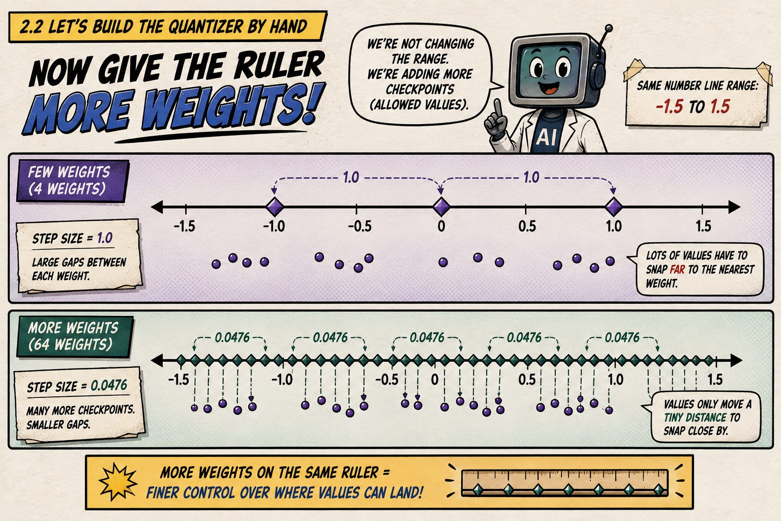
Here’s where the economics start to change.

Imagine that instead of six weights sharing this ruler, we had 64.

The original BF16 group would require:

64 weights × 16 bits
= 1,024 bits

The quantized codes would require:

64 weights × 2 bits
= 128 bits

We still need the same 32-bit ruler:

128 code bits + 32 ruler bits
= 160 bits total

Now compare the two:

Original BF16 group:     1,024 bits
Quantized group:           160 bits
Bits saved:                864 bits

That’s an 84.4% reduction:

864 ÷ 1,024
≈ 84.4%

And the complete group now has a compression ratio of:

1,024 ÷ 160
= 6.4 to 1

Nothing about the ruler changed. It still costs 32 bits. We’ve simply spread that fixed cost across many more weights.

You can visualize each group as a little box:

┌──────────────────────────────────────────────┐
│ 64 two-bit weight codes                     │
│ 128 bits                                    │
├──────────────────────────────────────────────┤
│ Shared minimum + scale                      │
│ 32 bits                                     │
└──────────────────────────────────────────────┘
Total: 160 bits

As the number of weights inside the box increases, the ruler becomes a smaller percentage of the total storage.

Assuming two BF16 ruler values per group, here’s what happens as we increase the number of weights sharing that ruler:

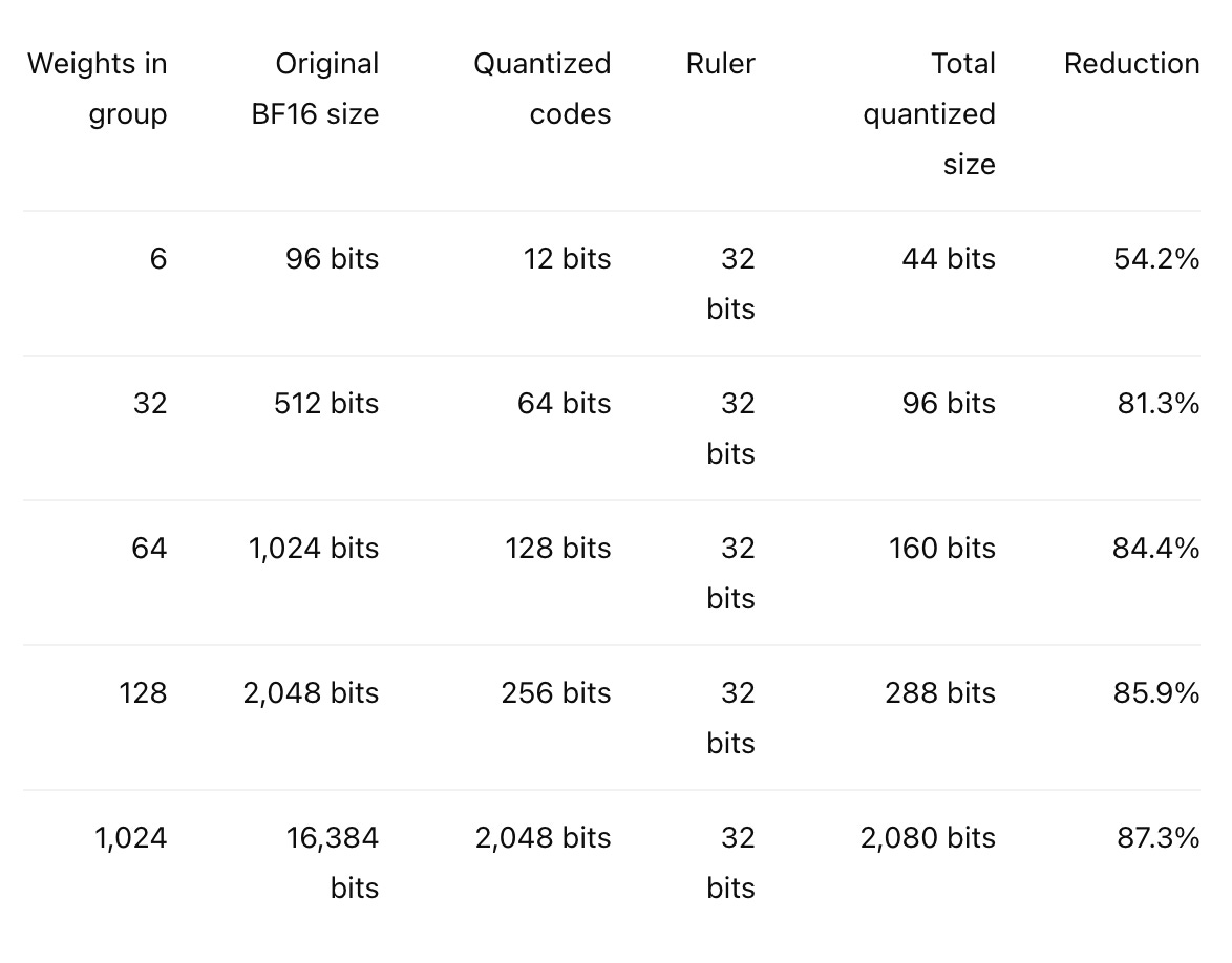
The theoretical maximum reduction from 16-bit to 2-bit storage is 87.5%. We can never quite reach that number because the ruler still takes up some space.

But as the group gets larger, we get closer and closer:

6 weights:         54.2% reduction
64 weights:        84.4% reduction
1,024 weights:     87.3% reduction
Infinite weights:  approaches 87.5%

The ruler hasn’t disappeared. Its cost has just become tiny relative to the number of weights using it.

Now we can write a formula that works for any group.

Let:

N = number of weights in the group
P = original bits per weight
Q = quantized bits per weight
M = metadata bits needed for the ruler

The original storage cost is:

original bits = N × P

The quantized storage cost is:

quantized bits = (N × Q) + M

The number of bits saved is:

bits saved = (N × P) - ((N × Q) + M)

And the percentage reduction is:

percentage saved
= 1 - quantized bits ÷ original bits

Putting everything together:

percentage saved
= 1 - ((N × Q) + M) ÷ (N × P)

For our 64-weight example:

N = 64
P = 16
Q = 2
M = 32

So:

percentage saved
= 1 - ((64 × 2) + 32) ÷ (64 × 16)
= 1 - 160 ÷ 1,024
= 84.375%

That formula gives us the memory reduction for one group.

A real model doesn’t usually place every weight under one enormous shared ruler. It splits the weights into many smaller groups, and every group gets its own scale and offset.

Let:

W = total number of weights
G = number of weights per group
Q = quantized bits per weight
M = metadata bits stored for each group

The number of groups is:

number of groups = ceil(W ÷ G)

We round up because a final partially filled group still needs its own ruler.

The total quantized storage is approximately:

total quantized bits
≈ (W × Q) + (ceil(W ÷ G) × M)

In plain English:

total quantized storage
≈ weight codes + all the shared rulers

For full groups, we can also express this as an effective number of bits per weight:

effective bits per weight
≈ Q + (M ÷ G)

That formula is incredibly useful.

For a 2-bit quantizer with 64 weights per group and 32 bits of metadata:

effective bits per weight
≈ 2 + (32 ÷ 64)
= 2.5 bits per weight

So even though we call it a 2-bit quantizer, the complete representation costs about 2.5 bits per weight once we include the ruler.

That’s the same basic phenomenon we saw with Unsloth’s GLM-5.2 files. The label tells us how aggressively the weights are being quantized, but the final file has a higher effective bits-per-parameter number because it also contains scales, metadata, higher-precision tensors and everything else required to make the model work.

Looking at the table, you might think we should let all 754 billion weights share a single ruler. The metadata cost would become basically zero, and we’d get incredibly close to the theoretical eightfold reduction.

Unfortunately, that would probably destroy the model.

One ruler has to cover the smallest and largest values inside its group. If that group contains weights with wildly different ranges or a few enormous outliers, our four diamonds get stretched across a huge section of the number line.

Most of the weights may then be forced into terrible approximations.

This gives us the first major tradeoff in quantization:

• Larger groups use less metadata and compress better.

• Smaller groups adapt more closely to local weight distributions and usually preserve more accuracy.

• Every quantizer has to choose where it wants to sit between those two.

So the goal isn’t simply to use as few bits as possible.

The goal is to use as few bits as possible without moving the important dots too far.

And now that we can calculate how far every dot moved, we can finally ask what those movements do to the model’s actual computations.

We now know how many bits we saved and how far each weight moved. But weights don’t sit inside a model waiting to be admired. They get multiplied by inputs.

So let’s put our cheap little approximations to work.

Take the six original weights from our toy model:

Original weights:
[-1.2, -0.7, -0.1, 0.3, 0.8, 1.4]

After quantization, they became:

Quantized weights:
[-1.2, -0.3333, -0.3333, 0.5333, 0.5333, 1.4]

Now imagine these six weights feeding into one tiny neuron.

Each weight has a corresponding input. The neuron multiplies each input by its weight and adds all six results together.

Visually, you can imagine six little streams flowing into one bucket:

input₁ × weight₁  ─┐
input₂ × weight₂  ─┤
input₃ × weight₃  ─┤
input₄ × weight₄  ─┼──→ add everything ──→ output
input₅ × weight₅  ─┤
input₆ × weight₆  ─┘

That operation is called a dot product.

Let’s make the first input as boring as possible:

input = [1, 1, 1, 1, 1, 1]

Because every input is 1, multiplying by the input doesn’t change any of the weights. The neuron’s output is just the sum of all six weights.

With the original weights:

output
= (1 × -1.2)
+ (1 × -0.7)
+ (1 × -0.1)
+ (1 × 0.3)
+ (1 × 0.8)
+ (1 × 1.4)
= -1.2 - 0.7 - 0.1 + 0.3 + 0.8 + 1.4
= 0.5

Now run the exact same input through the quantized weights:

quantized output
= (1 × -1.2)
+ (1 × -0.3333)
+ (1 × -0.3333)
+ (1 × 0.5333)
+ (1 × 0.5333)
+ (1 × 1.4)
≈ 0.6

The original neuron produced 0.5. The quantized neuron produced approximately 0.6.

So we moved four of the six weights, but the final output only moved by 0.1.

At first glance, that seems pretty encouraging. We compressed the weights dramatically, and the calculation barely changed.

But why did it barely change?

Let’s place each original weight directly underneath its quantized replacement:

Original:    [-1.2,  -0.7,    -0.1,   0.3,    0.8,    1.4]
Quantized:   [-1.2,  -0.3333,  -0.3333, 0.5333, 0.5333, 1.4]

Now subtract the original weight from the quantized weight:

error = quantized weight - original weight

That gives us an error vector:

[0, +0.3667, -0.2333, +0.2333, -0.2667, 0]

Picture each error as a little arrow.

Positive errors point to the right:

+0.3667  ───────→
+0.2333  ────→

Negative errors point to the left:

←────  -0.2333
←───── -0.2667

Our error vector contains arrows pointing in both directions:

0      +0.3667     -0.2333     +0.2333     -0.2667      0
•────────→          ←────•       •────→       ←────•      •

When every input equals 1, the neuron simply adds those arrows together.

The positive errors contribute:

+0.3667 + 0.2333 = +0.6

The negative errors contribute:

-0.2333 - 0.2667 = -0.5

So most of the movement cancels:

+0.6 + (-0.5) = +0.1

That is exactly the difference between our two outputs:

0.6 - 0.5 = 0.1

The individual weights moved by much more than 0.1. But some moved upward while others moved downward, and the final calculation only saw what was left after those errors fought each other.

This gives us our first important insight:

Large errors in individual weights don’t automatically create a large error in the final output. Some of those errors can cancel.

Unfortunately, they can also do the exact opposite.

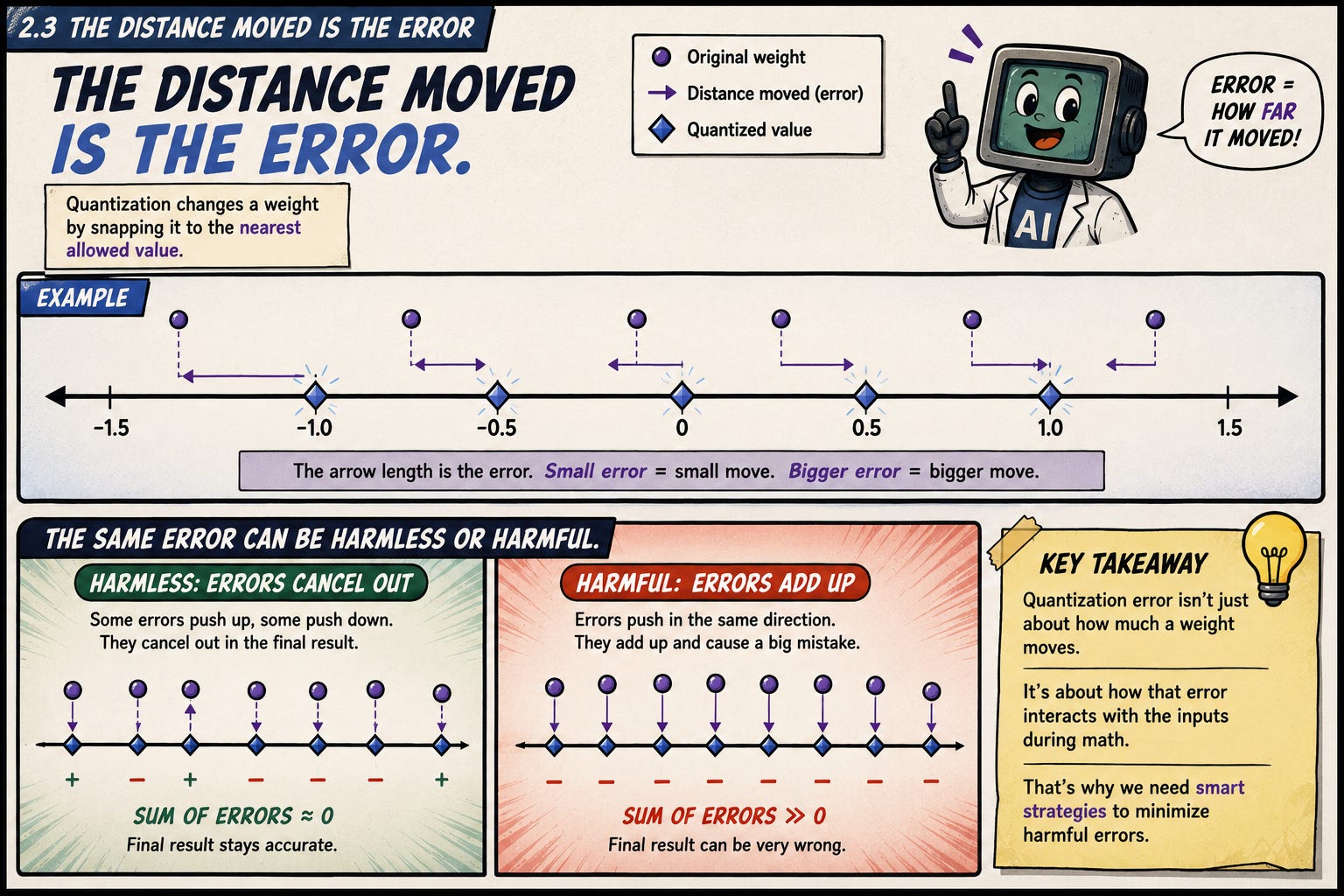
Keep the error vector exactly where it is:

[0, +0.3667, -0.2333, +0.2333, -0.2667, 0]

But now change the input:

input = [0, 1, -1, 1, -1, 0]

This input has been deliberately chosen to point in the same direction as our errors.

Where the error is positive, the input is positive. Where the error is negative, the input is negative. And because a negative number multiplied by another negative number becomes positive, all four errors now push the output in the same direction.

Let’s first calculate the output using the original weights:

original output
= (0 × -1.2)
+ (1 × -0.7)
+ (-1 × -0.1)
+ (1 × 0.3)
+ (-1 × 0.8)
+ (0 × 1.4)
= 0 - 0.7 + 0.1 + 0.3 - 0.8 + 0
= -1.1

Now use the quantized weights:

quantized output
= (0 × -1.2)
+ (1 × -0.3333)
+ (-1 × -0.3333)
+ (1 × 0.5333)
+ (-1 × 0.5333)
+ (0 × 1.4)
≈ 0

The original output was -1.1.

The quantized output is approximately 0.

Same weights. Same quantizer. Completely different response to the error.

With our first input, the quantization changed the output by only 0.1. With this input, it changed the output by roughly 1.1.

The quantized model didn’t suddenly become more damaged. We simply fed it an input that amplified the damage already present.

Let the original weights be a vector called:

w

Let the quantization error be:

e

Then the quantized weights are:

ŵ = w + e

If the input is x, the original output is:

y = w · x

The quantized output is:

ŷ = ŵ · x

Substitute w + e for the quantized weights:

ŷ = (w + e) · x

The dot product distributes across the addition:

ŷ = (w · x) + (e · x)

But w · x is just the original output:

ŷ = y + (e · x)

So the difference between the quantized and original outputs is:

output error = e · x

That’s the entire picture.

The error in the output isn’t determined by the quantization error alone. It’s determined by the interaction between the quantization error and the input flowing through the model.

A dot product can also be understood geometrically.

Picture the input vector x as one arrow and the error vector e as another. The dot product measures how much those arrows point in the same direction.

e · x = ||e|| × ||x|| × cos(θ)

Here, θ is the angle between the two arrows.

If the input points in roughly the same direction as the error, the dot product is large and positive:

error  ─────────→
input  ─────────→

If they point in opposite directions, the output error is large and negative:

error  ─────────→
input  ←─────────

If they’re perpendicular, the dot product is zero:

          input
            ↑
            |
error ──────→

The quantization error still exists, but that particular input doesn’t expose it.

This is why simply measuring how far the weights moved doesn’t tell us the whole story. Two quantizers can produce error vectors with the same overall size but behave very differently depending on where those errors point and which inputs the model actually sees.

Our toy neuron performed one dot product with six weights.

A real language model performs enormous matrix multiplications across layer after layer. The output from one layer becomes part of the input to the next.

So the process looks more like this:

input
  ↓
quantized matrix multiplication
  ↓
slightly changed activation
  ↓
next quantized matrix multiplication
  ↓
another changed activation
  ↓
another layer
  ↓
another layer
  ↓
token probabilities

The first layer doesn’t merely produce an incorrect final answer. It produces a slightly different intermediate representation.

That changed representation then flows into the next layer, where it interacts with another set of quantization errors. Some differences cancel. Some get dampened by normalization or nonlinearities. Others get amplified.

And occasionally, a small numerical change crosses a meaningful boundary.

It might change which token has the highest probability. In an MoE model, it might change which expert gets selected. In an attention layer, it might shift which earlier tokens receive the most attention.

The error doesn’t simply increase by a fixed amount in every layer. Neural networks are far messier than that. The effect depends on where the error occurs, what values are flowing through that part of the model and what calculations happen afterward.

But we can now see why some weights deserve more protection than others.

A weight that moves a little but rarely aligns with important inputs may not matter much. Another weight might move by the same amount and consistently distort a sensitive calculation.

That’s why great quantization isn’t just about minimizing the average distance between dots and diamonds.

It’s about figuring out which movements actually change what the model does.

Our handmade quantizer worked because the six weights we gave it were reasonably well behaved. They occupied a manageable range, and none of them wandered off to do something completely insane.

Real model weights aren’t always so cooperative.

Consider this slightly nastier set:

[-0.12, -0.08, -0.03, 0.02, 0.07, 0.11, 0.16, 4.00]

Put them on a number line and you get something like this:

● ●  ●  ● ● ● ●                                      ●
-0.12              0.16                              4.00

Seven weights are packed into a tiny region near zero. Then one asshole is sitting all the way out at 4.0.

Let’s quantize the entire group down to two bits.

Two bits gives us four representable levels. Our smallest value is -0.12, our largest is 4.0, and the full range is therefore:

4.0 - (-0.12) = 4.12

Four levels create three equal gaps, so the distance between each level becomes:

scale = 4.12 ÷ 3 ≈ 1.3733

That gives us the following ruler:

-0.12          1.2533          2.6267          4.00
  ◆---------------◆---------------◆---------------◆

Look at what just happened. Our first seven weights all live between -0.12 and 0.16, but the first jump on our ruler doesn’t occur until 1.2533.

Every one of those seven weights therefore gets pulled toward the same representable value:

-0.12 → -0.12
-0.08 → -0.12
-0.03 → -0.12
 0.02 → -0.12
 0.07 → -0.12
 0.11 → -0.12
 0.16 → -0.12
 4.00 →  4.00

The outlier survives perfectly. Everyone else gets flattened into a pancake.

The problem isn’t really that two bits gave us only four levels. The deeper problem is that we made eight very different weights share one ruler.

Most of that ruler is covering empty space:

useful values
┌───────┐
● ● ● ● ● ● ●
-0.12       0.16                    1.25          2.63          4.00
  ◆──────────┼────────────────────────◆─────────────◆─────────────◆
             enormous wasteland where no weights live

We’ve spent nearly all our available precision preserving the distance between one outlier and everything else.

The obvious fix is to stop forcing every weight to share the same ruler.

Suppose we split the values into two groups:

Group A: [-0.12, -0.08, -0.03, 0.02]
Group B: [0.07, 0.11, 0.16, 4.00]

Group A now gets a ruler covering only -0.12 to 0.02.

scale = (0.02 - (-0.12)) ÷ 3 ≈ 0.0467

Its four representable levels become:

-0.1200      -0.0733      -0.0267       0.0200
   ◆-------------◆-------------◆-------------◆

That gives us much closer approximations:

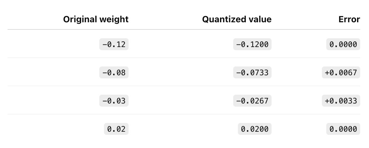
Beautiful. Our ruler actually fits the numbers it’s trying to measure.

Group B still has a problem, though:

[0.07, 0.11, 0.16, 4.00]

Its ruler has to stretch from 0.07 to 4.0, so the first three values will still collapse toward the same level.

We could split it again:

Group B1: [0.07, 0.11, 0.16]
Outlier:  [4.00]

Now the smaller values get their own tight ruler, while 4.0 can be handled separately or kept at higher precision.

That improves accuracy, but we’re not getting those extra rulers for free.

Remember what each group needs to store:

• The low-bit codes representing its weights

• A scale telling us how far apart the representable levels are

• Sometimes an offset or zero point telling us where the ruler begins

Let’s assume each scale and offset together require 32 bits.

If all eight weights share one group, the storage looks like this:

8 weights × 2 bits = 16 bits of codes
1 shared ruler      = 32 bits of metadata
Total               = 48 bits

The original BF16 weights required:

8 weights × 16 bits = 128 bits

So the one-group version shrinks the storage from 128 bits to 48 bits, a reduction of 62.5%.

Now give the weights two separate rulers:

8 weights × 2 bits = 16 bits of codes
2 shared rulers     = 64 bits of metadata
Total               = 80 bits

We still save space, but the reduction falls to 37.5%.

More rulers usually give us better approximations. They also eat into our compression.

LARGER GROUPS                                      SMALLER GROUPS
less metadata                                      more metadata
better compression                                 weaker compression
rougher local fit                                  better local fit

And now we can finally attach the annoying technical vocabulary to what we’ve been doing.

Imagine this small weight matrix:

[ 0.1  0.2  0.3  0.4  3.8  4.0  4.2  4.4 ]
[ 1.0  1.1  1.2  1.3  7.6  7.8  8.0  8.2 ]

The quantization strategy determines which of these weights have to share the same ruler.

Per-tensor quantization gives the entire matrix one ruler:

[ 0.1  0.2  0.3  0.4  3.8  4.0  4.2  4.4 ]
[ 1.0  1.1  1.2  1.3  7.6  7.8  8.0  8.2 ]
  └──────────── one ruler: 0.1 to 8.2 ────────────┘

That ruler has to cover everything from 0.1 to 8.2. If we only have four representable levels, they’ll be spread across that entire range.

That’s bad news for the small values. Numbers like 0.1, 0.2, 0.3 and 0.4 may all get rounded to the same level.

Per-tensor quantization is simple and requires very little metadata. But one unusual region of the tensor can distort the ruler for everything else.

Per-channel quantization gives each complete row, column or channel its own ruler. The exact direction depends on how the tensor is organized and used.

For this simplified example, we’ll treat each row as a channel:

[ 0.1  0.2  0.3  0.4  3.8  4.0  4.2  4.4 ]  ruler A: 0.1 to 4.4
[ 1.0  1.1  1.2  1.3  7.6  7.8  8.0  8.2 ]  ruler B: 1.0 to 8.2

We now have two rulers instead of one. The second row’s values no longer force the first row’s ruler to stretch all the way to 8.2.

But each ruler still covers an entire channel. Within the first row, the values around 0.1 are still sharing a ruler with values around 4.4.

That’s where group-wise quantization goes further.

Group-wise quantization chops each channel into smaller blocks:

[ 0.1  0.2  0.3  0.4 | 3.8  4.0  4.2  4.4 ]
  └── ruler A ───────┘   └── ruler B ───────┘
[ 1.0  1.1  1.2  1.3 | 7.6  7.8  8.0  8.2 ]
  └── ruler C ───────┘   └── ruler D ───────┘

Now the first four weights get a ruler from 0.1 to 0.4, while the next four get one from 3.8 to 4.4.

That’s meaningfully different from per-channel quantization. Instead of one ruler per entire row, we have multiple rulers inside each row.

Real quantizers might use groups of 32, 64 or 128 consecutive weights. Smaller groups let each ruler fit its local values more closely, but every additional ruler requires more metadata.

Mixed-precision quantization changes the number of bits we spend on different parts of the model.

Suppose testing shows that these three groups tolerate aggressive rounding:

[ 0.1  0.2  0.3  0.4 ]  → 2 bits per weight
[ 3.8  4.0  4.2  4.4 ]  → 2 bits per weight
[ 1.0  1.1  1.2  1.3 ]  → 2 bits per weight

But the final group turns out to be unusually important:

[ 7.6  7.8  8.0  8.2 ]  → 8 bits per weight

Mixed precision lets us compress the tolerant groups aggressively while giving the sensitive group more room.

The group boundaries and the bit widths are two separate choices:

• Group-wise quantization decides which weights share a ruler.

• Mixed-precision quantization decides how many representable levels each group receives.

This is the core idea behind recipes like Unsloth’s dynamic quantization. A model labeled “1-bit” doesn’t necessarily store every single weight using exactly one bit. More tolerant areas can be pushed toward extremely low precision, while fragile areas remain at higher precision.

The word “dynamic” can make this sound like the model is changing precision every time it generates a token. That’s not necessarily what’s happening. In this context, it’s better to think of the quantization recipe as treating different parts of the model differently when the quantized file is created.

Some tensors can take the full low-bit beating. Others can’t.

And that means quantization isn’t really asking whether the entire model can survive at one bit.

It’s asking two much more useful questions:

1. Which weights should have to share the same ruler?

2. How many bits should we spend on each group?

We’ve now spent an obscene amount of time learning how quantization works from the ground up.

We’ve turned weights into tiny codes. We’ve built rulers. We’ve packed multiple codes into a single byte. And we’ve seen why forcing wildly different weights to share the same ruler can completely flatten the information they contain.

Now we can return to the result that started this whole article and look at it with slightly more educated eyes.

GLM-5.2 contains roughly 754 billion parameters. Its BF16 version is approximately 1.51 TB.

Unsloth produced several quantized versions, including:

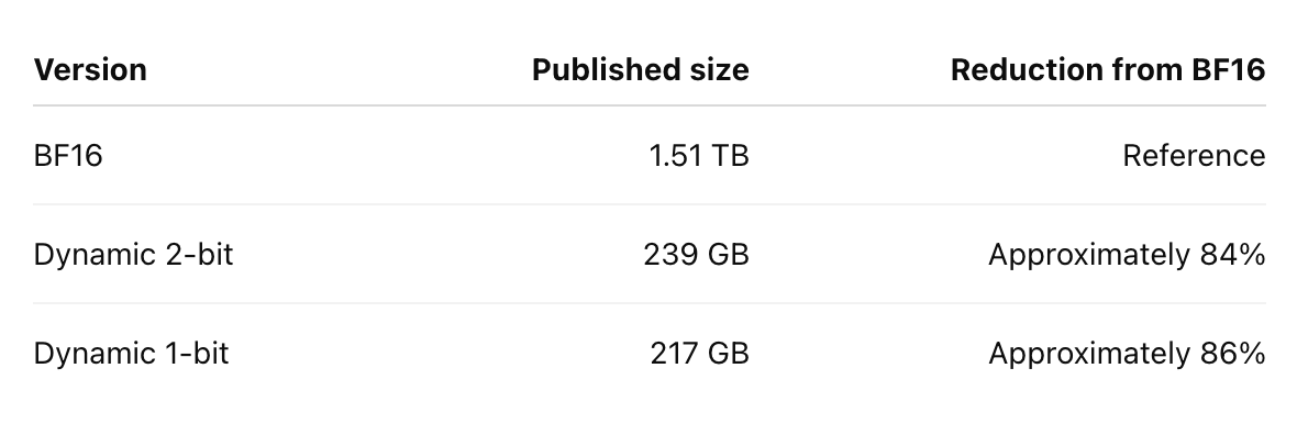
That’s the headline.

Unsloth took something that ordinarily requires around a terabyte and a half of weight storage and squeezed it into a few hundred gigabytes.

But the actual file sizes contain our first clue about how they did it.

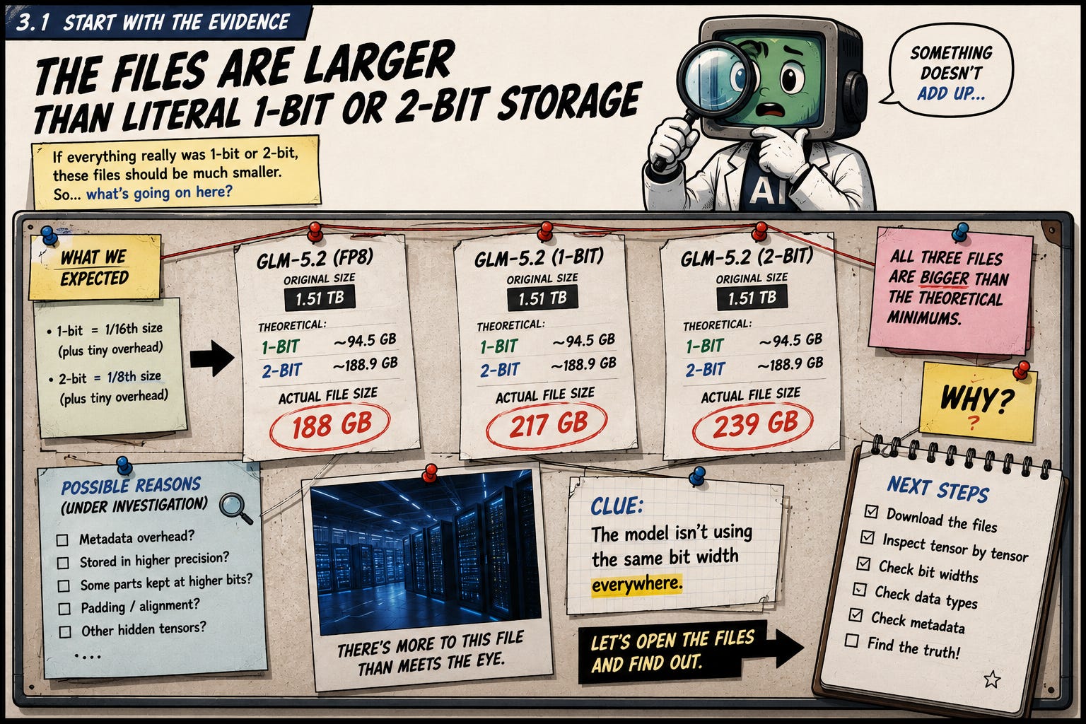
Start with the simplest possible interpretation of “two-bit model.”

GLM-5.2 has roughly 754 billion parameters. If every parameter were stored using exactly two bits, the raw weights would require:

754 billion parameters × 2 bits
= 1.508 trillion bits

Eight bits make one byte:

1.508 trillion bits ÷ 8
≈ 188.5 billion bytes
≈ 188.5 GB

So the theoretical two-bit floor looks like this:

Literal 2-bit weights:
[===============================] 188.5 GB

But Unsloth’s Dynamic 2-bit file is approximately:

[========================================] 239 GB

That leaves roughly 50.5 GB beyond the literal two-bit weight payload:

239 GB - 188.5 GB = 50.5 GB

Now repeat the calculation for one bit:

754 billion parameters × 1 bit ÷ 8
≈ 94.25 GB

The theoretical one-bit floor is tiny:

Literal 1-bit weights:
[===============] 94.25 GB

But Unsloth’s Dynamic 1-bit file is approximately:

[===================================] 217 GB

That’s more than twice the size of the literal one-bit weight payload.

This doesn’t mean anything is wrong.

It means the words “one-bit” and “two-bit” are summaries of the quantization approach, not literal descriptions of every byte inside the finished file.

The file still needs information such as:

• The packed low-bit weight codes

• The scales used to reconstruct approximate weights

• Other block-level quantization metadata

• Tensor names, shapes and model metadata

• Values that aren’t stored using the headline bit width

That final point is important, but it’s still a hypothesis until we inspect the recipe more carefully. The file sizes strongly suggest that the finished models contain more than uniformly packed one-bit or two-bit weights, but the headline sizes alone can’t tell us exactly how those extra bytes are divided.

They give us a clue, not the complete answer.

There’s another way to look at the same clue.

We can take the total file size and spread it evenly across all 754 billion parameters:

effective bits per parameter
≈ file size × 8 ÷ parameter count

For the 239 GB version:

239 × 8 ÷ 754
≈ 2.54 effective bits per parameter

For the 217 GB version:

217 × 8 ÷ 754
≈ 2.30 effective bits per parameter

This does not mean Unsloth invented a tiny physical container capable of holding exactly 2.30 bits.

The average is combining several different things:

low-bit codes
      +
scales and metadata
      +
potential higher-precision values
      │
      ▼
average storage cost

Think of it like averaging the spending at a restaurant.

One person ordered water. Another ordered pasta. Somebody else got the lobster and made an aggressive number of visits to the cocktail menu.

Nobody spent exactly the average amount. But the average still tells us what the table cost as a whole.

In the same way, 2.30 effective bits per parameter tells us the average storage cost of the completed 1-bit package. It doesn’t tell us the precision of each individual tensor.

That distinction matters because it opens the door to a much more interesting possibility:

Some tensors  → extremely low precision
Some tensors  → slightly more precision
Some tensors  → significantly more protection

Instead of distributing bits evenly across the model, Unsloth may be distributing them according to where they’re most valuable.

We can’t prove the exact allocation from the file size alone.

But we now know what kind of allocation could explain it.

Of course, making a model smaller isn’t impressive by itself.

I can reduce GLM-5.2 to zero bytes using one extremely advanced compression technique called “deleting it.”

What made Unsloth’s result interesting was that the compressed models still produced outputs resembling the BF16 reference.

Unsloth says it used KL divergence to evaluate its GLM-5.2 quantizations. It also reported approximately:

• 82% top-token agreement for Dynamic 2-bit

• 76.2% top-token agreement for Dynamic 1-bit

We’ll unpack those measurements properly in a moment.

For now, imagine giving the same prefix to both models:

"The capital of France is"

Each model produces a probability distribution over the possible next tokens:

                         ┌── BF16 distribution
Same prefix ─────────────┤
                         └── Quantized distribution

If quantization had destroyed the model, those distributions would bear little resemblance to each other.

The BF16 model might strongly favor "Paris", while the quantized model sprays probability across unrelated tokens.

Instead, Unsloth’s measurements suggest that the aggressively quantized versions retain a meaningful amount of the reference model’s next-token behavior.

So we need to explain two things at once:

The model became dramatically smaller
                AND
The model still behaved meaningfully like BF16

Uniformly crushing every tensor to the lowest possible precision explains the first result.

It probably doesn’t explain the second.

At this point, we can divide our evidence into three buckets.

• GLM-5.2 contains roughly 754 billion parameters.

• Its BF16 version is approximately 1.51 TB.

• Unsloth publishes Dynamic 1-bit and 2-bit versions around 217 GB and 239 GB.

• Those files are larger than literal uniform one-bit and two-bit weight storage would predict.

• Unsloth reports meaningful similarity between the quantized models and the BF16 reference.

• The finished files contain more than naked low-bit weight codes.

• Different kinds of values may be receiving different amounts of precision.

• The quantization recipe probably pays special attention to which parts of the model are sensitive.

• Scales, grouping and other metadata contribute materially to the file size.

• The exact precision assigned to every tensor

• The precise method used to identify sensitive parts

• The grouping and scaling decisions used throughout the model

• The calibration data used to make those decisions

• How much each individual technique contributed to the final quality

That final category is where our experiment begins.

We’re not going to pretend we can recreate Unsloth’s internal recipe perfectly from a file listing and a Hugging Face post. That would be bullshit.

What we can do is start with the dumbest possible quantizer and keep asking the same three questions:

1. HOW SMALL DID IT GET?
   Count the packed weights, scales and metadata.
2. HOW CLOSE IS IT TO BF16?
   Compare probability distributions and top-token choices
   while both models receive identical token prefixes.
3. CAN IT STILL DO USEFUL WORK?
   Compare completed answers across factual questions,
   instruction following, structured output and code.

Each test looks at a different layer of the result.

A tiny model can be useless.

A model can disagree with BF16 while still producing a perfectly good answer.

And a model can look statistically similar across ordinary text while quietly losing its ability to write code or call tools.

That’s why we’ll need all three tests.

But before we can test a clever quantization recipe, we need a stupid baseline.

So we’re going to give every eligible tensor the same two-bit treatment, see what survives and then work backward from whatever breaks.

We don’t need to quantize a tiny, unrelated model and pretend it tells us what Unsloth did to GLM-5.2.

We can inspect the actual artifacts.

Unsloth publishes the BF16 model alongside multiple quantized versions in its GLM-5.2 GGUF repository. The Dynamic 2-bit model, for example, is split across six GGUF files totaling approximately 239 GB.

A GGUF file isn’t just a bucket of anonymous compressed numbers. It contains a directory describing the model:

GGUF FILE
│
├── Model architecture
├── Tensor names
├── Tensor dimensions
├── Tensor quantization types
├── Tokenizer information
├── Model configuration
└── Packed tensor data

That tensor directory is basically our autopsy report.

It lets us ask which parts of GLM-5.2 were pushed into extremely low-bit formats and which parts received more protection.

A simplified tensor inventory might look like this:

blk.0.attn_q.weight
blk.0.attn_k.weight
blk.0.attn_v.weight
blk.0.attn_output.weight
blk.0.ffn_gate_exps.weight
blk.0.ffn_up_exps.weight
blk.0.ffn_down_exps.weight
blk.0.ffn_gate_inp.weight
output.weight
token_embd.weight

Each tensor also carries a storage type.

If the whole model had been uniformly quantized, we’d expect to see roughly the same low-bit type everywhere:

Attention tensor        → IQ2
Expert tensor           → IQ2
Router tensor           → IQ2
Embedding tensor        → IQ2
Output tensor            → IQ2

A dynamic quantization should look more like a patchwork:

Large tolerant tensors  → extremely low precision
Sensitive tensors       → higher precision
Tiny critical tensors   → possibly left mostly intact

We shouldn’t invent the exact tensor-by-tensor map without dumping every shard’s metadata. But Unsloth’s own documentation confirms the broader idea: Dynamic 2.0 uses a model-specific quantization scheme, and the layers treated differently in one model can differ significantly from those protected in another.

So “Dynamic 2-bit” isn’t one blunt setting applied evenly across GLM-5.2.

It’s a model-specific precision map.

The repository also contains a file called imatrix_unsloth.gguf_file.

It’s approximately 1.13 GB.

That file isn’t part of the model users load for ordinary inference. It’s an importance matrix used while producing the quantized model.

The basic idea is surprisingly intuitive.

Suppose one row of weights is multiplied by an activation vector:

weights      ×      activations      =      output
[w₁ w₂ w₃]         [a₁]                    y
                   [a₂]
                   [a₃]

After quantization, the weights move slightly:

w₁ → q₁
w₂ → q₂
w₃ → q₃

The change in the output depends on both the weight error and the activation:

output error
≈ (q₁ - w₁)a₁
+ (q₂ - w₂)a₂
+ (q₃ - w₃)a₃

If a₁ is almost always tiny, moving w₁ may barely matter.

If a₂ is constantly huge, the same amount of rounding on w₂ can have a much larger effect.

Visually:

Weight error × tiny activation
              │
              ▼
        tiny output change
Weight error × huge activation
              │
              ▼
        huge output change

The importance matrix records information about how strongly different weight directions are used when representative data flows through the model.

The implementation used by llama.cpp approximates this using activation statistics. Instead of treating every rounding error equally, the quantizer places a larger penalty on errors attached to frequently or strongly activated directions.

So the ruler is no longer asking:

Which representable value is numerically closest to this weight?

It’s asking something closer to:

Which rounding choice creates the least damage when this weight is actually used?

That’s a much better question.

To build the importance matrix, Unsloth runs calibration data through the unquantized model and observes its activations.

Its Dynamic 2.0 documentation says its newer calibration dataset contains more than 1.5 million tokens, depending on the model, and includes hand-curated and cleaned data intended to better represent conversational behavior.

Conceptually:

Calibration prompts
        │
        ▼
Run the original model
        │
        ▼
Observe which channels activate
        │
        ▼
Build importance matrix
        │
        ▼
Quantize important directions carefully

The calibration data matters because the model only reveals which internal pathways it uses in response to the examples it sees.

If the calibration set contains only Wikipedia articles, the quantizer may become very good at preserving the parts of the model used for Wikipedia-style text.

That doesn’t guarantee it preserves the parts needed for code, tool calls or long conversations.

Unsloth explicitly warns about this problem. Its documentation says text-only calibration data can be a poor fit for instruction models and notes that evaluating on data too similar to the calibration set can make a quant look artificially strong.

That gives us another clue about the recipe:

Unsloth isn’t only choosing a quantization format. It’s choosing which behavior the quantizer should try hardest to preserve.

We don’t have Unsloth’s exact GLM-5.2 command or complete tensor-by-tensor decision rule.

But the public artifacts let us reconstruct the overall process:

1. Start with BF16 GLM-5.2
              │
              ▼
2. Run more than 1.5M calibration tokens
              │
              ▼
3. Record activation importance
              │
              ▼
4. Build the 1.13 GB importance matrix
              │
              ▼
5. Quantize large weight groups aggressively
              │
              ▼
6. Protect sensitive tensors or layers
              │
              ▼
7. Package the mixed result into GGUF
              │
              ▼
8. Compare it with BF16

The llama.cpp quantization tooling supports exactly the kinds of controls this would require:

• Supplying an importance matrix

• Assigning different quantization types to specific tensors

• Protecting the token embedding or output tensors

• Applying tensor rules by name or layer pattern

That doesn’t prove which exact flags Unsloth used. It shows that the GGUF format and tooling can express the kind of mixed-precision model its public documentation describes.

GLM-5.2 is a mixture-of-experts model.

Most of its enormous parameter count lives inside expert weight matrices. Only a subset of those experts is activated for any given token.

That creates a very tempting precision budget.

If the giant expert tensors can tolerate extreme compression, pushing them toward one or two bits saves a massive amount of storage. Smaller but more sensitive components can then remain at higher precision without moving the total file size nearly as much.

Imagine the model’s storage as a budget:

GLM-5.2 PARAMETER MASS
MoE expert tensors:
[=====================================================]
Everything else:
[=====]

Saving one bit across the enormous expert region produces a huge reduction.

Spending several extra bits on a much smaller router, normalization tensor or attention component may barely change the final file size.

This doesn’t prove which GLM-5.2 tensors Unsloth protected. We need the complete tensor map for that.

But it explains how mixed precision can preserve important behavior without giving back most of the storage savings.

Crush the enormous tolerant region
                 +
Protect the smaller sensitive region
                 =
Very small model that still works

So our current best reconstruction is:

Unsloth used a large, model-specific calibration dataset to observe how GLM-5.2 actually uses its internal weights. It recorded those activation patterns in an importance matrix, used that information to reduce damaging rounding choices and applied different quantization treatment across the model rather than forcing every tensor into one uniform bit width.

That interpretation is supported by:

• The published Dynamic 2.0 documentation

• The model-specific quantization claim

• The 1.13 GB importance-matrix file

• The finished model sizes

• The mixed quantization capabilities exposed by the GGUF tooling

What we still don’t have is the exact GLM-5.2 precision map.

We can’t yet say:

This exact tensor used one bit.
This exact tensor used four bits.
This exact tensor remained in BF16.

But we can say something more meaningful than “Unsloth made it smaller.”

They appear to have used calibration data to decide where precision was valuable, then spent their available bits accordingly.

The next question is whether the result still behaves like the original model.

And that’s where KL divergence, top-token agreement and real task testing come in.

At this point, we’ve established that Unsloth made GLM-5.2 much smaller. That part isn’t really up for debate. You can see the files. You can count the bytes. The model went from roughly 1.5 TB in BF16 to 217 GB for the dynamic 1-bit version and 239 GB for the dynamic 2-bit version.

The harder question is whether the model survived the trip.

And this is much harder to answer than it initially sounds. A language model doesn’t store a neat list of answers that we can compare before and after quantization. It takes a sequence of tokens, performs an unholy amount of math and produces a probability distribution for what might come next.

Quantization changes some of that math. The changes may be tiny, but they happen across hundreds of billions of weights and flow through layer after layer. By the time we reach the output, the model’s probability distribution may have moved.

The obvious response is to ask whether the model still gives the right answers. But even that skips over a few important layers of the problem.

Before testing the final answer, we need to understand what changed inside the prediction process. That means asking three progressively more practical questions:

1. Did the probability distribution move?

2. Did that movement change the winning token?

3. Did the completed task actually get worse?

Each question catches something the others miss. So let’s take them one at a time.

Suppose we give the original BF16 model this sentence:

The capital of France is...

The model doesn’t immediately reach into a database and retrieve “Paris.” Instead, it assigns a probability to every possible next token in its vocabulary.

That vocabulary might contain more than 100,000 tokens. But to keep this readable, let’s pretend it contains only five possibilities.

The BF16 model might produce something like this:

BF16
Paris       ███████████████████  94%
Lyon        ▌                     2%
London      ▎                     1%
France      ▎                     1%
Other       ▌                     2%

The model strongly prefers Paris. Depending on our sampling settings, Paris will almost certainly become the next token.

Now let’s feed the exact same sentence into the quantized model:

QUANTIZED
Paris       ██████████████████   89%
Lyon        █                      4%
London      ▌                      2%
France      ▌                      2%
Other       ▊                      3%

The quantized model also chooses Paris.

If we only checked the winner, we’d say nothing changed. Both models got the answer right.

But something did change.

                 BF16      QUANTIZED
Paris             94%  ─────→  89%
Lyon               2%  ─────→   4%
London             1%  ─────→   2%
France             1%  ─────→   2%
Other              2%  ─────→   3%

A little probability moved away from Paris and spread across the other options.

That movement may be harmless. Paris still wins by an absurd margin. But we shouldn’t assume every change will be this gentle. In another context, the top two tokens might already be nearly tied. A small shift could change which token wins and send the generation down a different path.

So our first job isn’t to ask whether the answer changed. It’s to measure how much the entire probability distribution moved.

For that, we need something called KL divergence.

KL divergence has one of those names that makes a fairly intuitive idea sound like it requires three graduate degrees.

It doesn’t.

At its core, KL divergence compares two probability distributions. In our case, it compares the original BF16 model’s predictions with the quantized model’s predictions.

We’ll call the BF16 distribution P and the quantized distribution Q.

Before touching the formula, imagine both models are placing bets on the next token:

BF16 MODEL                 QUANTIZED MODEL
cat       ██████  60%      cat       █████   50%
dog       ███     30%      dog       ████    40%
rabbit    █       10%      rabbit    █       10%

Both models think “cat” is most likely. The quantized model is simply a little less confident about it and a little more interested in “dog.”

KL divergence gives us a way to summarize all that movement with one number.

More specifically, it asks:

How surprised would I be if I used the quantized model’s probabilities while expecting the BF16 model’s behavior?

The formula looks like this:

KL(P || Q) = Σ P(i) × log(P(i) / Q(i))

That looks unpleasant, so let’s slow it down.

For every possible token, we take the probability assigned by BF16 and compare it with the probability assigned by the quantized model.

• i represents one possible token.

• P(i) is BF16’s probability for that token.

• Q(i) is the quantized model’s probability.

• P(i) / Q(i) compares the two bets.

• log turns that comparison into a manageable penalty.

• Multiplying by P(i) makes tokens BF16 cared about matter more.

• Σ tells us to repeat the process for every token and add everything together.

Conceptually, we’re doing this:

Choose one token
      │
      ▼
Compare BF16 and quantized probabilities
      │
      ▼
Measure how far the probabilities moved
      │
      ▼
Weight the change by BF16's confidence
      │
      ▼
Repeat for every token and add everything

The weighting is important.

If BF16 assigns a token a probability of 0.0001%, the quantized model moving that probability around probably doesn’t matter very much.

But if BF16 assigns a token a probability of 60% and the quantized model drops it to 10%, we should care. Something the original model strongly believed has nearly disappeared.

If both models assign a token exactly the same probability, the ratio between them is one:

P(i) / Q(i) = 1

And because:

log(1) = 0

That token contributes nothing to the divergence.

BF16             QUANTIZED
rabbit  10%  ─── rabbit  10%
No movement
No surprise
No KL penalty

Now let’s compare two complete distributions.

Our BF16 model produces:

cat       ██████  60%
dog       ███     30%
rabbit    █       10%

The quantized model produces:

cat       █████   50%
dog       ████    40%
rabbit    █       10%

The numbers aren’t identical, but the overall shape remains similar. Both models prefer cat, dog remains second and rabbit remains a distant third.

The resulting KL divergence is approximately:

KL ≈ 0.023

That’s small.

Now imagine the quantized model produces this instead:

BF16                         QUANTIZED
cat       ██████  60%        cat       █       10%
dog       ███     30%        dog       ████    40%
rabbit    █       10%        rabbit    █████   50%

This time, most of the probability has moved away from cat and toward rabbit.

The resulting KL divergence is approximately:

KL ≈ 0.828

That’s much larger.

KL = 0
Identical distributions
KL = 0.023
Small movement
KL = 0.828
Large movement

The exact number isn’t meaningful in isolation. There isn’t a universal KL score below which every model is magically safe. We care about how divergence changes across quantization methods, token positions and real datasets.

The intuition is what matters:

KL divergence measures the extra surprise created when we use the quantized model’s probability distribution as a substitute for BF16’s.

There’s also one technical wrinkle worth mentioning. KL divergence is directional:

KL(P || Q) isn’t necessarily equal to KL(Q || P).

We aren’t measuring a perfectly symmetrical distance between two models. We’re specifically treating BF16 as our reference and asking how well the quantized model approximates it.

That’s why the order matters.

Now that we know what we’re measuring, we need to be careful about how we run the test.

If we let both models generate complete responses, they may choose different tokens early on.

The BF16 model might generate:

The capital of France is Paris, which is...

The quantized model might generate:

The capital of France is located in...

Neither continuation is necessarily wrong. But the models are now reading different text.

SHARED PREFIX
The capital of France is
             │
        ┌────┴────┐
        ▼         ▼
      Paris     located
        │         │
        ▼         ▼
      which       in

Once the paths split, every later prediction is conditioned on a different prefix.

If their probability distributions diverge after that, we won’t know why. Quantization might have damaged the model, or the models might simply be completing different sentences.

To isolate the effect of quantization, both models need to see the same prefix at every step.

Shared prefix
     │
     ├──→ BF16 distribution
     │
     └──→ Quantized distribution
                 │
                 ▼
          Compare predictions
                 │
                 ▼
        Reveal the actual next token
                 │
                 ▼
          Extend shared prefix
                 │
                 └──→ Repeat

This is sometimes called teacher forcing. Instead of allowing each model’s chosen token to become its next input, we keep feeding both models the same known sequence.

Both models stay on the same road. We’re comparing how they would’ve predicted each turn without allowing one early disagreement to contaminate everything afterward.

Run this across millions of token positions and we get a distribution of KL values. We can see where quantization barely changes anything and where it seriously distorts the model’s internal bets.

But KL divergence still isn’t the entire story.

A probability distribution can move without changing the winning token. So next, we need to ask how often the winner itself changes.

Top-token agreement ignores everything except the most likely next token.

The question is simply:

Did BF16 and the quantized model choose the same winner?

This is the metric featured in Unsloth’s GLM-5.2 results.

According to Unsloth:

DYNAMIC 1-BIT     217 GB     76.2% top-token agreement
DYNAMIC 2-BIT     239 GB     82.0% top-token agreement

The dynamic 2-bit model chose the same highest-probability token as BF16 about 82% of the time under Unsloth’s evaluation.

That’s extremely impressive for a model that’s roughly one-sixth the original size.

But we need to be precise about what the number means.

It doesn’t mean the quantized model retained exactly 82% of its intelligence. It doesn’t mean it’ll score 82% as well on every benchmark. And it doesn’t mean the remaining 18% of its choices were necessarily wrong.

It only means a different token occupied the top spot.

Here’s an example:

BF16                         QUANTIZED
large      ██████  31%       large      ██████  29%
massive    ██████  29%       massive    ██████  30%
enormous   ████    18%       enormous   ████    18%
Winner: large                Winner: massive

BF16 chooses “large.”

The quantized model chooses “massive.”

That counts as a top-token disagreement even though the distributions are almost identical and either token may produce an equally good sentence.

Now compare that with this:

BF16                         QUANTIZED
Paris      ██████████ 94%    Paris      ██      18%
London     ▎           2%    London     ██████  61%
Winner: Paris                Winner: London

That’s also one top-token disagreement.

But clearly, it’s a much scarier one.

SAME METRIC RESULT
large → massive      Top-token disagreement
Paris → London       Top-token disagreement
VERY DIFFERENT CONSEQUENCES

The metric treats these cases equally even though one is a harmless synonym swap and the other is the model confidently relocating France.

That makes top-token agreement incomplete. But it doesn’t make it a bad metric.

In fact, a strong top-token agreement number is an extremely encouraging directional signal. Given the same prefix, the quantized model is repeatedly arriving at the exact same immediate decision as BF16.

Think about what has to remain intact for that to happen.

The weights have been heavily compressed. Numerical errors have been introduced throughout the model. Those errors flow through layer after layer of matrix multiplication. And despite all that, the quantized model still ranks the same token first across a large majority of the tested prefixes.

That suggests the model’s learned decision boundaries have largely survived.

SAME PREFIX
     │
     ├──→ BF16 model ─────────→ "Paris"
     │
     └──→ Quantized model ────→ "Paris"
Same context
Different numerical precision
Same final token

If that happens across millions of prefixes, it’s strong evidence that quantization hasn’t completely scrambled the model’s behavior.

We should still be careful, though. An 82% top-token agreement rate doesn’t mean 82% of complete generations will be identical.

Language models are autoregressive. Every generated token becomes part of the next prefix. One early disagreement can send two otherwise similar models down different paths.

SAME PREFIX
     │
     ├──→ "large"   → "model" → "can" → "handle"...
     │
     └──→ "massive" → "model" → "is"  → "able"...

The responses may quickly stop matching token for token even when they continue expressing essentially the same idea.

Top-token agreement is therefore best understood as a measure of local behavioral preservation.

Given the same context, how often does the quantized model make the exact same immediate decision as BF16?

A high number is very good news. It means the compressed model is reproducing the original model’s local behavior across a large number of contexts.

It just doesn’t tell us how serious the remaining disagreements are.

We can learn more by examining the tokens involved in each disagreement.

One possible approach is to represent both tokens as vectors and calculate their cosine similarity.

A token embedding is basically a long list of numbers describing where that token sits in the model’s learned representation space. Tokens used in similar ways tend to point in similar directions.

Cosine similarity measures the angle between those vectors:

cosine similarity = (A · B) / (||A|| × ||B||)

We don’t need to unpack every symbol right now. The useful intuition is:

Similarity near 1       Vectors point in similar directions
Similarity near 0       Vectors are mostly unrelated
Similarity near -1      Vectors point in opposite directions

If BF16 chooses “large” and the quantized model chooses “massive,” their token vectors should generally point in similar directions.

large    ───────────────→
massive  ──────────────→
Nearly the same direction
High cosine similarity
Probably a mild disagreement

If BF16 chooses “large” and the quantized model chooses “banana,” the vectors should be much farther apart.

large  ───────────────→
banana
   │
   ▼
Different directions
Low cosine similarity
Probably a more serious disagreement

This gives us a rough way to divide disagreements into buckets:

SAME TOP TOKEN
Exact agreement
DIFFERENT TOKEN + HIGH VECTOR SIMILARITY
Likely a related word, synonym or formatting variation
DIFFERENT TOKEN + LOW VECTOR SIMILARITY
Potentially a meaningful behavioral change

Instead of reporting only the percentage of exact matches, we could examine the entire disagreement set.

How many involved highly similar tokens? How many jumped into completely different semantic territory? How much probability did BF16 assign to the replacement? How far down BF16’s original ranking was that token?

That final question is especially useful.

Suppose BF16 ranks “large” first at 31% and “massive” second at 29%. If quantization flips them, the selected token changed, but the quantized model chose something BF16 already considered extremely plausible.

BF16 RANKING
1. large       31%
2. massive     29%   ← Quantized model chose this
3. enormous    18%

That’s very different from the quantized model selecting something BF16 ranked 8,000th with effectively zero probability.

BF16 RANKING
1. Paris        94%
2. Lyon          2%
3. France        1%
...
8,417. banana    0.00001%   ← Quantized model chose this

Both are top-token disagreements. The second represents a much larger departure from BF16’s behavior.

Vector similarity gives us one view of severity. BF16’s ranking and probability give us another.

But vector similarity has its own limitation.

“Paris” and “London” may be relatively close in embedding space. They’re both cities, capitals, European locations and proper nouns. A vector-similarity test may describe the substitution as semantically mild.

Paris   ───────────────→
London  ──────────────→
Similar concepts
High vector similarity
Still factually wrong

Semantic similarity isn’t the same as correctness.

So a stronger analysis combines several signals:

TOP-TOKEN AGREEMENT
Did the winner stay the same?
          │
          ▼
VECTOR SIMILARITY
If not, were the two tokens semantically related?
          │
          ▼
BF16 RANK AND PROBABILITY
Did BF16 already consider the replacement plausible?
          │
          ▼
CONTEXTUAL OR TASK EVALUATION
Did the substitution preserve meaning and correctness?

This gives us a much richer interpretation of Unsloth’s result.

An 82% top-token agreement rate means the dynamic 2-bit model exactly reproduced BF16’s immediate decision across a large majority of the tested prefixes.

For the remaining 18%, we shouldn’t automatically label every disagreement a failure. Some may be tiny ranking flips between nearly interchangeable tokens. Others may produce different wording while preserving the same meaning. And yes, some may represent actual damage.

The headline agreement number tells us that the quantized model is directionally behaving a lot like the original.

The disagreement analysis tells us how worried we should be about the places where it doesn’t.

Eventually, we have to stop staring at probability distributions and ask the annoyingly practical question:

Does the model still work?

If you’re evaluating a coding model, give it a repository. Ask it to fix a bug. Run the tests.

If you’re evaluating a tool-using model, let it use the tools. Check whether it selected the right tool, produced valid arguments and recovered when something failed.

If you’re evaluating structured output, validate the JSON instead of admiring how philosophically similar its logits appear.

PROBABILITY DISTRIBUTION
Did the model's internal bets move?
              │
              ▼
TOP-TOKEN AGREEMENT
Did that movement change the winner?
              │
              ▼
DISAGREEMENT SEVERITY
How different was the replacement?
              │
              ▼
TASK EVALUATION
Did the completed work get worse?

The useful task-level tests depend on what you’re actually serving:

• Does the generated code compile?

• Do the unit tests pass?

• Is the JSON valid?

• Did the model call the correct tool?

• Is the mathematical answer correct?

• Did the agent complete the workflow?

• How often did a human have to intervene?

• How many tokens, seconds and dollars did success require?

This is where quantization can get weird.

A model might preserve ordinary writing almost perfectly while becoming worse at exact arithmetic. It might remain excellent at short code completion but become less reliable across long agentic workflows. It might preserve benchmark performance while becoming slightly more repetitive or brittle.

Average KL divergence may not expose those failures. Top-token agreement and vector similarity may not expose them either.

They emerge when the model has to complete an entire task.

There’s one final complication.

The data used to decide which weights deserve additional precision shouldn’t be the same data used to prove that the finished model works.

Otherwise, we end up doing this:

Calibration prompts
        │
        ▼
Choose which weights to protect
        │
        ▼
Evaluate on the same prompts
        │
        ▼
Amazing-looking result

We’ve taught the quantization process exactly which errors will appear on the test.

What we actually want is:

CALIBRATION DATA                 TEST DATA
Choose precision                Measure quality
Protect sensitive weights       Test unseen prompts
Tune the quantizer               Run real tasks
          SEPARATE DATASETS

This is the same basic reason we separate training data from test data everywhere else in machine learning.

Unsloth’s Dynamic 2.0 documentation says its process uses a curated calibration dataset containing more than 1.5 million tokens. That data helps identify which parts of the model are sensitive and should receive more precision.

The final evaluation should use different prompts and tasks.

Otherwise, we’re letting the quantizer peek at the answer key and then acting shocked when it crushes the exam.

Now we can finally take everything we’ve learned and apply it to the actual models.

Start with the size difference:

APPROXIMATE MODEL SIZE
BF16          ██████████████████████████████  1,508 GB
2-bit         █████                             239 GB
1-bit         ████                              217 GB

The 2-bit version removes roughly 1.27 TB from the original BF16 footprint.

That’s the difference between needing several expensive pieces of hardware and potentially fitting the model inside one large unified-memory system.

But size means nothing if the model no longer works. So now add behavioral preservation:

TOP-TOKEN AGREEMENT
1-bit         ███████████████       76.2%
2-bit         ████████████████      82.0%
                                      ▲
                                +5.8 percentage points

The 2-bit model is only 22 GB larger than the 1-bit model.

That’s roughly a 10% increase in file size in exchange for a 5.8-point improvement in exact top-token agreement.

Imagine evaluating both models across 10,000 fixed token positions:

1-bit agrees with BF16 about 7,620 times
2-bit agrees with BF16 about 8,200 times
Additional exact matches from 22 GB: about 580

Those 580 additional matches don’t automatically translate into 580 corrected answers. Some of the original disagreements may have been harmless.

But every additional match removes one opportunity for the quantized model to leave BF16’s immediate path.

Because generation is autoregressive, preventing an early divergence can matter far beyond one token.

One additional agreement
          │
          ▼
Same next prefix
          │
          ▼
More comparable next prediction
          │
          ▼
Less opportunity for the generations to split

That makes the extra 22 GB look like a fantastic trade if both versions fit comfortably on the same hardware.

There’s another revealing clue inside the file sizes.

If all 754 billion parameters were stored using exactly one bit, the weights would theoretically occupy about 94 GB.

But Unsloth’s 1-bit file is 217 GB.

A perfectly uniform 2-bit representation would theoretically occupy about 189 GB. Unsloth’s 2-bit file is 239 GB.

                    THEORETICAL      ACTUAL FILE
Uniform 1-bit          94 GB            217 GB
Uniform 2-bit         189 GB            239 GB

That additional space isn’t a mistake.

It’s the strategy.

The files need scales, offsets, metadata and other structural information. More importantly, Unsloth isn’t forcing every part of the model to use the same precision.

Some tensors can tolerate brutal compression. Others are sensitive enough that rounding them aggressively may cause disproportionate damage.

So “dynamic 1-bit” describes the broad strategy. It doesn’t mean every number is represented by exactly one bit.

Using the headline sizes, the 1-bit version averages roughly 2.30 effective bits per parameter. The 2-bit version averages roughly 2.54.

Dynamic 1-bit     ≈ 2.30 effective bits per parameter
Dynamic 2-bit     ≈ 2.54 effective bits per parameter

That difference is tiny.

The 2-bit model spends only about one-quarter of an additional bit per parameter on average, but gains 5.8 points of top-token agreement.

This is the larger lesson behind dynamic quantization.

The goal isn’t to treat every weight fairly. The goal is to spend bits where they preserve the most useful behavior.

TOLERANT WEIGHTS              SENSITIVE WEIGHTS
Compress aggressively         Preserve more precision
Save lots of memory           Prevent major damage
               ONE MIXED MODEL

Based on the published results, we can confidently say that both models preserve a surprisingly large amount of BF16’s local behavior.

The dynamic 1-bit version is an incredible technical demonstration. Compressing a 754-billion-parameter model to 217 GB while retaining 76.2% exact top-token agreement is fucking wild.

The dynamic 2-bit model looks like a stronger deployment candidate. It gives up only 22 GB while improving agreement to 82%.

But the published agreement numbers don’t tell us everything.

We still don’t know the KL-divergence distribution. We don’t know how many disagreements are harmless ranking flips. We don’t know how semantically similar the disagreeing tokens are. And we don’t yet have enough evidence here about coding, mathematics, tool use or long agentic workflows.

THE REMAINING 18% IN THE 2-BIT MODEL
Tiny ranking flips
        +
Synonym substitutions
        +
Different but valid phrasing
        +
Factually meaningful mistakes
        +
Completely broken predictions

Top-token agreement tells us the size of that bucket.

KL divergence, vector similarity, BF16 ranking and task evaluation would tell us what’s inside it.

So we shouldn’t claim the 239 GB model is identical to BF16.

It almost certainly isn’t.

But we also shouldn’t look at an 18% disagreement rate and conclude that it lost 18% of its intelligence. That isn’t what the metric means.

If I were serving GLM-5.2, I’d begin by testing the 2-bit version.

The extra 22 GB is relatively small compared with the model’s overall size. In return, we get meaningfully higher agreement with BF16 and fewer opportunities for numerical error to push generation down another path.

There is one major exception.

Those 22 GB may push the deployment across a hard memory boundary.

A 239 GB model doesn’t leave much room on a 256 GB system for runtime overhead, temporary buffers and the KV cache. If the 2-bit version requires another machine or SSD offloading while the 1-bit model fits cleanly, the infrastructure difference may outweigh the quality improvement.

IF BOTH FIT COMFORTABLY
Choose 2-bit
Better behavioral preservation
Small relative memory increase
IF 2-BIT CROSSES A MEMORY BOUNDARY
Test 1-bit seriously
Lower agreement may be worth avoiding
another device or SSD offloading

That’s what makes quantization an infrastructure decision rather than merely a model-quality decision.

I think Unsloth’s result is genuinely huge.

It doesn’t prove that we can shrink every model to 1-bit without consequences. It doesn’t prove that benchmarks, coding agents and long-running workflows remain untouched. And it definitely doesn’t eliminate the need for proper evaluation.

But it does show that the relationship between model size and useful behavior is much more flexible than the original BF16 checkpoint makes it appear.

The 1-bit version demonstrates the outer edge of compression.

The 2-bit version looks like a more balanced exchange between memory and preserved behavior.

And both suggest that a massive portion of the original 1.5 TB footprint wasn’t equally important.

THE OLD ASSUMPTION
More numerical precision
          =
More useful intelligence
WHAT THESE RESULTS SUGGEST
Preserve precision selectively
          +
Compress everything else aggressively
          =
Most of the behavior at a fraction of the size

A 1.5 TB model doesn’t necessarily need 1.5 TB of memory to remain useful.

It may need only 239 GB, a very clever quantization strategy and a willingness to figure out which numerical details actually matter.

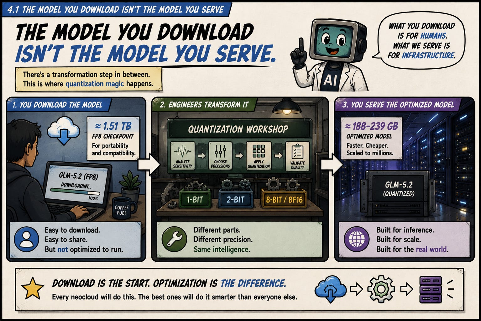
Let’s zoom out for a second and imagine that you’ve downloaded an enormous open model.

If you’re running it for yourself, your goal is pretty simple. You need to find enough memory to load the weights, start the runtime and generate tokens at a speed you can tolerate. If it takes a few minutes to load or occasionally crashes, that’s annoying, but nobody’s calling your support team.

A neocloud has a completely different problem. It needs to serve that same model to hundreds or thousands of people, handle many requests at once and maintain enough spare capacity that the service doesn’t fall over whenever somebody pastes in a giant repository.

The model’s weights are only the beginning of the memory bill.

PRODUCTION MEMORY
Model weights
      +
KV cache
      +
Runtime buffers
      +
Concurrent requests
      +
Operational headroom

All of that has to fit inside a finite amount of fast memory.

As we covered in my obscenely long article about inference memory, the weights don’t disappear after the model starts. The hardware repeatedly reads them while generating tokens, so they need to remain close to the processors doing the math.

For a model as large as GLM-5.2, that creates a fairly brutal starting point.

The model contains roughly 754 billion parameters. If we momentarily ignore scales, metadata and other overhead, we can estimate the weight footprint by multiplying those 754 billion parameters by the number of bits used to store each one.

THEORETICAL WEIGHT STORAGE
BF16     16 bits per weight     ≈ 1,508 GB
FP8       8 bits per weight     ≈   754 GB
4-bit     4 bits per weight     ≈   377 GB
2-bit     2 bits per weight     ≈   189 GB
1-bit     1 bit per weight      ≈    94 GB

The number of parameters never changes in this example. GLM-5.2 remains a roughly 754-billion-parameter model at every row in the table.

What changes is how much information we use to represent each parameter.

Moving from BF16 to FP8 saves roughly 754 GB before we’ve removed a single weight. Moving from FP8 to 4-bit saves another 377 GB.

That isn’t a cute optimization around the edges. It can change the physical shape of the entire deployment.

LARGER WEIGHT FOOTPRINT
More accelerator memory
        │
        ▼
More devices per model replica
        │
        ▼
More cross-device communication
        │
        ▼
More expensive inference
SMALLER WEIGHT FOOTPRINT
Fewer devices per replica
        │
        ▼
Less communication
        │
        ▼
More room for users and KV cache
        │
        ▼
Cheaper inference

This is where quantization stops being an interesting compression trick and becomes a business requirement.

Imagine that an inference provider manages to fit one copy of GLM-5.2 across a collection of GPUs.

That’s a real technical accomplishment. The model is loaded, the endpoint works and users can send requests.

But one running copy of the model isn’t necessarily enough to operate a real service.

A production provider may need multiple replicas to support more simultaneous requests, absorb sudden demand and keep the endpoint alive when a device or server fails. It may also maintain separate pools for different regions, context lengths or service tiers.

Every additional replica requires another copy of the model’s weights.

So every byte occupied by the checkpoint gets multiplied across the fleet.

ONE 754 GB REPLICA
████████████████████  754 GB

One replica ties up roughly 754 GB of theoretical weight memory at FP8.

Now imagine that demand requires four replicas:

FOUR 754 GB REPLICAS
████████████████████  754 GB
████████████████████  754 GB
████████████████████  754 GB
████████████████████  754 GB
Total weight memory: about 3,016 GB

The same model weights now occupy just over 3 TB of fast memory across the fleet.

Now let’s cut the weight representation from eight bits to four:

FOUR 377 GB REPLICAS
██████████  377 GB
██████████  377 GB
██████████  377 GB
██████████  377 GB
Total weight memory: about 1,508 GB

The model didn’t gain any new knowledge. It didn’t become more intelligent and it still contains roughly the same number of parameters.

But the provider just recovered about 1.5 TB of fast memory across four theoretical replicas.

That memory can now be used to create additional replicas, support larger batches, accept longer prompts or maintain more KV cache. It can also allow the provider to use fewer devices for each replica and avoid some of the communication that happens when a model is split across hardware.

In other words, the provider can turn that recovered memory into more capacity.

And more capacity means more paying customers on the same hardware.

This is where the memory problem gets even more annoying.

The model’s weights aren’t the only thing consuming memory. Every active request creates a KV cache that stores information about the tokens the model has already processed. That cache grows as the prompt and generated response become longer.

So a neocloud is constantly dividing its available memory between the model itself and the people trying to use it.

TOTAL AVAILABLE MEMORY
┌────────────────────────────────────────────┐
│              MODEL WEIGHTS                 │
├────────────────────────────────────────────┤
│        KV CACHE + ACTIVE REQUESTS           │
├────────────────────────────────────────────┤
│       BUFFERS + OPERATIONAL HEADROOM        │
└────────────────────────────────────────────┘

If the weights occupy nearly all the available memory, the model may technically fit while leaving very little room to serve requests.

That’s the difference between getting a checkpoint to load and getting a production endpoint to work.

MODEL FITS
"Look, it generated a token!"
PRODUCTION FITS
"Look, it generated tokens for hundreds of users
without running out of memory or collapsing!"

The first result is exciting when you’re experimenting locally.

The second result is the actual job of a neocloud.

Every gigabyte removed from the weights becomes a gigabyte that might support more context, another active request or a larger batch. That can increase the number of customers served by the same hardware and reduce the provider’s cost per token.

The model’s memory footprint therefore doesn’t just determine whether inference is possible. It determines how economically useful the hardware can become.

This leads us to a slightly strange conclusion.

The checkpoint released by the model creator isn’t necessarily the model an inference provider should serve in production.

It’s raw material.

The model creator usually needs to publish weights in a format that works across a reasonably broad range of hardware and software. It can’t perfectly optimize one public checkpoint for every accelerator, runtime and customer workload.

An inference provider has a much narrower problem. It knows what hardware it owns, which numerical formats that hardware accelerates and which runtime will execute the model. It also has a much better view into the actual workloads its customers are sending.

That changes the optimization target.

MODEL CREATOR'S CHECKPOINT
Broad compatibility
General-purpose precision
Portable release format
            │
            ▼
     INFERENCE PROVIDER
            │
            ├── Hardware-specific format
            ├── Workload-specific calibration
            ├── Custom kernels
            ├── Quality validation
            └── Deployment-specific quantization
            │
            ▼
PRODUCTION MODEL

The provider can ask questions the model creator couldn’t answer universally.

Which tensors can be compressed safely on this exact model? Which numerical format runs fastest on this exact hardware? Which errors matter for our customers? Does the model need to preserve creative writing, tool use, code generation or all three?

Once you see the problem this way, quantization becomes much more than downloading a smaller GGUF file from Hugging Face.

The provider has to choose a representation that fits its hardware and then prove that the resulting model still works for its customers.

The same public checkpoint can therefore become several different production models.

This is exactly what Baseten did with GLM-5.2.

Z.ai released GLM-5.2 using FP8 weights. Baseten wanted to serve the model on NVIDIA Blackwell hardware, which includes tensor cores designed to accelerate NVFP4 operations.

So Baseten didn’t simply load the original checkpoint and expose an API around it.

It performed an in-house conversion from FP8 to NVFP4 using NVIDIA ModelOpt.

Z.ai GLM-5.2
Original FP8 weights
        │
        ▼
Baseten calibration data
        │
        ▼
In-house NVFP4 quantization
        │
        ▼
Quality testing on agent workloads
        │
        ▼
Blackwell-optimized production endpoint

The quantization reduced the precision of the affected weights from eight bits to four.

For one number, that difference looks almost comically small:

ONE WEIGHT
FP8       8 bits      ████████
NVFP4     4 bits      ████

But GLM-5.2 doesn’t contain one weight. It contains hundreds of billions of them.

When a four-bit saving is repeated across that much parameter mass, it becomes hundreds of gigabytes of theoretical memory reduction.

That means less data needs to sit in VRAM and less weight data needs to travel through memory during inference. Blackwell can also execute NVFP4 operations through hardware designed specifically for that format.

So the same quantization can attack multiple bottlenecks at once:

NVFP4 QUANTIZATION
Smaller weight representation
          │
          ├──→ Less VRAM capacity required
          │
          ├──→ Less pressure on VRAM bandwidth
          │
          └──→ Faster Blackwell tensor-core operations

The obvious problem is that Baseten could’ve made the model faster by making it worse.

Cutting the numerical precision changes the weights. As we spent the first three parts of this article establishing, those changes can alter probability distributions, change top-token decisions and eventually damage completed tasks.

Baseten therefore couldn’t simply perform the conversion and assume everything survived.

It calibrated and tested the quantized model around common patterns for agents. It then compared the NVFP4 version with the original FP8 model using the BFCL function-calling benchmark.

According to Baseten, the two versions produced scores within the benchmark’s margin of error.

That doesn’t mean every probability or generated token remained identical.

It means Baseten compressed the representation, unlocked faster execution and still preserved the practical function-calling behavior it cared about closely enough that the benchmark couldn’t establish a meaningful difference.

ORIGINAL FP8 MODEL             QUANTIZED NVFP4 MODEL
Larger weights                 Smaller weights
More VRAM traffic              Less VRAM traffic
Baseline execution             Faster Blackwell execution
        │                               │
        └──────── Roughly equivalent ───┘
               BFCL performance

This is precisely the trade every serious inference provider is going to chase.

Not the smallest model at any cost.

Not the fastest model after destroying its ability to reason.

The goal is the smallest and fastest representation that still completes the customer’s workload reliably.

Now imagine three providers all advertising GLM-5.2.

The first serves the original weights.

The second downloads a generic quantization created by someone else.

The third builds its own calibration dataset, protects the tensors that matter for its customers and quantizes the rest into a format designed specifically for its hardware.

                    GLM-5.2
                       │
        ┌──────────────┼──────────────┐
        ▼              ▼              ▼
   Provider A      Provider B      Provider C
Original weights  Generic quant   Custom quant
Generic runtime   Smaller model   Workload-tuned
More memory       Better fit      Hardware-specific
        │              │              │
        ▼              ▼              ▼
 Different cost, speed, capacity and quality

All three companies can put “GLM-5.2” on their pricing pages.

But they won’t have the same cost per token. They may not support the same number of concurrent users, achieve the same speed or preserve the same model behavior.

The model name tells you which underlying intelligence they started with.

It doesn’t tell you how efficiently they turned that model into a production service.

This is why a neocloud can’t treat quantization as an optional afterthought.

For sufficiently large models, serving the original weights can waste too much scarce memory. But blindly choosing the smallest available quantization can damage the model enough to make the savings pointless.

The provider has to find the useful point between those extremes.

TOO MUCH PRECISION
Great quality
Terrible memory economics
TOO LITTLE PRECISION
Great memory economics
Terrible model quality
THE PRODUCTION TARGET
Maximum compression
without meaningful workload damage

The provider that gets this balance right can serve more users with the same hardware while preserving the quality people came for.

The provider that gets it wrong either pays for memory it didn’t need or serves a cheaper model that quietly became worse.

That makes the model creator’s checkpoint the starting point.

For a neocloud, the production model is something it increasingly has to build for itself.

This creates another problem for neoclouds.

Once a provider decides that serving the original checkpoint is too expensive, it still has to decide which quantization to use.

At first, this sounds like a simple size-versus-quality decision. A 4-bit model should preserve more information than a 2-bit model, while the 2-bit model should require less memory.

The provider could seemingly choose the smallest version that reaches an acceptable benchmark score and move on with its life.

Unfortunately, models don’t break that cleanly.

A quantization can perform extremely well on one kind of workload and quietly become worse on another. The errors introduced by rounding depend partly on which weights become important while the model processes a particular input.

That means the “best” quantization depends on what people will ask the model to do.

SAME ORIGINAL MODEL
General chat
Code generation
Function calling
Mathematics
Long-context reasoning
Creative writing
        │
        ▼
Different activations
Different sensitive weights
Different acceptable errors

A provider serving coding agents may care deeply about exact syntax, function names and structured tool calls.

A provider serving casual chat may care more about conversational quality, factuality and natural wording.

A provider serving legal or financial analysis may care about long-context retrieval and precise numerical reasoning.

The same compressed model may not preserve all of those behaviors equally well.

To understand why, return to the tiny quantizer we built earlier.

Quantization replaces a highly precise weight with a nearby approximation.

ORIGINAL WEIGHT       QUANTIZED WEIGHT
0.4187        →       0.4000

The error looks tiny:

0.4187 - 0.4000 = 0.0187

But that weight doesn’t operate alone. During inference, it gets multiplied by an activation.

output contribution = weight × activation

If the activation is small, the rounding error barely matters.

0.0187 × 0.1 = 0.00187

If the activation is large, the same rounding error becomes much more important.

0.0187 × 100 = 1.87

The quantized weight didn’t change between these examples.

The input did.

SAME QUANTIZATION ERROR
Small activation       →       Tiny output error
Large activation       →       Large output error

Different prompts create different activation patterns. A coding prompt may strongly activate one collection of weights, while a creative-writing prompt leans on another.

So a quantization that looks excellent on ordinary conversation may still damage the pathways needed for code, mathematics or tool use.

That’s why calibration data matters.

A post-training quantizer doesn’t simply need access to the weights. It also needs representative inputs.

The provider runs those inputs through the original model and observes how its internal activations behave. Those observations help identify which tensors, channels or groups are especially sensitive to rounding.

CALIBRATION PROMPTS
        │
        ▼
Run through original model
        │
        ▼
Observe activation patterns
        │
        ▼
Identify sensitive weights and tensors
        │
        ▼
Assign precision and scaling rules

The calibration data is effectively showing the quantizer which parts of the model matter for the workloads it expects to encounter.

If the calibration set contains code, tool definitions and agent trajectories, the quantization has a chance to protect the model’s behavior on those inputs.

If it contains only simple conversational prompts, the quantizer may never discover that a particular tensor becomes especially important during repository-scale coding.

The quantizer can only optimize around the behavior it actually sees.

CHAT-HEAVY CALIBRATION
Conversation
Summarization
Question answering
        │
        ▼
Protect behavior commonly activated by chat
CODING-HEAVY CALIBRATION
Source code
Tool calls
Repository context
Bug fixes
        │
        ▼
Protect behavior commonly activated by coding

This doesn’t mean the resulting model can only perform the calibration tasks. It still contains the same underlying architecture and parameter count.

It means the compression decisions are informed by one view of how the model will be used.

If that view is badly wrong, the quantizer may protect the wrong things.

This is why a generic benchmark score can be dangerously comforting.

Suppose a provider quantizes a coding model and evaluates it on a collection of short factual questions. The score barely changes.

That’s useful evidence, but it doesn’t prove that the model can still edit a repository, preserve a JSON schema or call a tool with the correct arguments.

QUANTIZED MODEL
Great score on trivia
        │
        ▼
Provider declares victory
        │
        ▼
Customer asks it to modify a repository
        │
        ▼
Model produces syntactically valid nonsense

The evaluation needs to resemble the work customers will actually submit.

For a coding-focused neocloud, that might include:

• Generating code that compiles

• Fixing bugs against real test suites

• Editing several related files

• Navigating large repositories

• Preserving exact function and variable names

• Producing valid tool calls

• Maintaining coherence through long agent workflows

For a general agent platform, the tests may focus more heavily on function selection, argument construction, instruction following and recovery after tool failures.

For a long-context provider, the model needs to retrieve the correct information from enormous prompts without quietly losing accuracy near the middle.

CUSTOMER WORKLOAD
        │
        ▼
Representative calibration data
        │
        ▼
Workload-aware quantization
        │
        ▼
Matching task evaluation

The calibration data teaches the quantizer what behavior matters.

The evaluation data determines whether that behavior survived.

And as we discussed earlier, those should be separate datasets. Otherwise, the quantizer gets to study the same examples used to prove that it works.

This is why the Baseten example from the previous section is so revealing.

Baseten didn’t only say that it converted GLM-5.2 from FP8 to NVFP4. It said that its calibration and testing focused on common patterns for agents.

It then evaluated the quantized model on BFCL, a benchmark centered around function calling.

BASETEN'S TARGET
Production agent workloads
        │
        ▼
Agent-focused calibration
        │
        ▼
NVFP4 quantization
        │
        ▼
Function-calling evaluation

The calibration target, deployment target and evaluation target all point in roughly the same direction.

That doesn’t prove the NVFP4 model is perfect across every possible use case. It gives Baseten evidence that the quantization preserved the behavior required for the product it wanted to operate.

That’s a much more useful claim.

The important question isn’t:

Did quantization preserve everything equally?

It’s:

Did quantization preserve the things our customers are paying us to do?

Push this logic far enough and an interesting possibility appears.

A neocloud may not end up with one universally optimal quantization for each model. It may maintain different versions for different hardware, workloads or service tiers.

ONE ORIGINAL CHECKPOINT
          │
          ├──→ Coding-optimized quantization
          │
          ├──→ General-chat quantization
          │
          ├──→ Maximum-quality quantization
          │
          └──→ Maximum-throughput quantization

The coding version might protect tensors that become sensitive during code generation and tool use.

The general-chat version might optimize for broad language quality.

A high-quality tier might use more bits and occupy more devices.

A high-throughput tier might accept a modest quality reduction in exchange for dramatically lower cost.

The provider could then route each request toward the model representation that best matches the user’s needs.

INCOMING REQUEST
"What does this function do?"
          │
          ▼
Coding-optimized quantization
"Write me a wedding toast"
          │
          ▼
General-language quantization

This doesn’t mean the precision changes magically inside one loaded checkpoint every time a request arrives.

The provider would maintain separate quantized artifacts or deployment pools and route requests between them.

That adds operational complexity. Every additional version needs memory, validation, monitoring and its own deployment process.

But it also creates another optimization lever.

The provider no longer has to force every customer and workload through one numerical representation.

The original model may be open. Anyone can download the same checkpoint.

But the calibration dataset, precision map, kernel implementation and evaluation process don’t have to be open.

PUBLIC
Original model weights
Architecture
Tokenizer
PROVIDER-SPECIFIC
Calibration data
Tensor-level precision choices
Hardware-specific kernels
Quality thresholds
Workload evaluations
Routing strategy

Two providers can begin with identical weights and end up with different production quality, throughput and cost.

The difference isn’t the intelligence of the original model.

It’s how effectively each provider compresses and serves it.

Quantization therefore isn’t merely a preprocessing step that every neocloud performs once. It becomes an ongoing engineering discipline.

Every new model has different sensitive tensors. Every new hardware generation accelerates different numerical formats. Every customer workload produces different activation patterns. And every additional bit of compression creates another trade between memory and behavior.

New model released
        │
        ▼
Profile target workloads
        │
        ▼
Build calibration set
        │
        ▼
Generate quantized candidates
        │
        ▼
Run task-specific evaluations
        │
        ▼
Deploy the best trade
        │
        ▼
Monitor real customer behavior
        │
        └──→ Improve and repeat

The downloadable checkpoint gives every provider the same starting point.

The quantization recipe helps determine who can turn it into the best service.

You knew this was coming eventually.

This workload-specific approach is a core part of the bet we’re making at CueCloud.

We’re building specifically for coding and agentic workloads. That means we don’t just care whether a quantized model can answer trivia or write a decent poem. We care whether it can navigate a repository, produce valid tool calls, preserve structured output and keep its shit together through a long coding workflow.

Those are the behaviors our calibration data and evaluations need to protect.

OPEN MODEL CHECKPOINT
        │
        ▼
Coding and agent calibration
        │
        ▼
Hardware-aware quantization
        │
        ▼
Repository and agent evaluations
        │
        ▼
CueCloud production model

Our broader bet is that we can combine excellent open models, aggressive but careful quantization and memory-heavy hardware to serve coding workloads without forcing every token through the most expensive HBM-equipped GPU available.

Quantization is what makes that bet possible.

If we can shrink a model enough to fit comfortably on cheaper hardware while preserving the coding behavior people actually care about, we don’t just reduce the size of a file. We change the economics of serving the model.

BETTER QUANTIZATION
Less memory per model
        │
        ▼
More capacity from each machine
        │
        ▼
Lower cost per completed coding task
        │
        ▼
More tokens without terrifying usage bills

That last point is the actual product.

Developers don’t wake up wanting a beautifully calibrated mixed-precision checkpoint. They want capable models, fast responses and enough usage that they don’t have to nervously watch a token meter while an agent reads half their repository.

The quantization work stays underneath.

The cheaper, more predictable access is what the customer gets.

Phew.

That was a lot.

We started with a viral post about Unsloth squeezing GLM-5.2 into dynamic 1-bit and 2-bit files. From there, we somehow ended up talking about floating-point numbers, rulers, buckets, activation patterns, KL divergence, token embeddings, calibration datasets and the economics of operating a neocloud.

So if your brain currently feels slightly quantized itself, I get it.

But the core idea is much simpler than all the machinery surrounding it.

A model is an enormous collection of learned numbers. Those numbers don’t all need to be stored with the same level of precision, and they definitely don’t all deserve the same share of our very expensive memory.

THE BET BEHIND QUANTIZATION
Preserve precision where it matters
          +
Compress aggressively where it doesn't
          =
Most of the useful behavior
at a fraction of the memory

Doing this badly is easy. You can round every weight aggressively, produce a beautifully tiny model file and completely destroy the behavior people wanted from it.

Doing it well is much harder. You need to understand where quantization error appears, which parts of the model are sensitive and whether the resulting changes actually damage the completed task.

That’s what makes Unsloth’s work so exciting. It isn’t just that the files are small. It’s that the published top-token agreement suggests a surprising amount of GLM-5.2’s original behavior survived.

And Baseten shows the other half of the story. Custom quantization isn’t limited to researchers and people running enormous models on weird hardware in their basements. It’s already becoming part of how serious inference providers turn public checkpoints into economically viable services.

There’s still plenty we didn’t cover.

There are rotation-based methods, quantization-aware training, curvature-based approaches, better ways of handling outliers and a whole universe of hardware-specific kernels that determine whether a compressed model is actually faster.

I’ll get into all of that another day because this article is already long enough and we all have families.

For now, I hope this made quantization feel a little less like magical model shrinkage and a little more like what it really is:

A careful decision about which numerical details are worth paying to preserve.

If we keep getting better at making that decision, some of the world’s largest models may become dramatically cheaper and easier to serve without becoming dramatically worse.

And that’s a pretty fantastic promise.