Finding a book through Reinforcement Learning

Lately I was studying some fundamental reinforcement learning algorithms, and as I was sitting in the library in Schöneberg I was thinking about what I could implement to see them in practice. The idea that came to me was a small example where an agent tries to find a book in a bookshelf. So I built a small gridworld, a procedurally generated library with some rows of shelves, one door in, one book somewhere in the stacks, and the goal of finding it. I wanted something small enough to show me what the trade-offs actually look like instead of just reading about them.

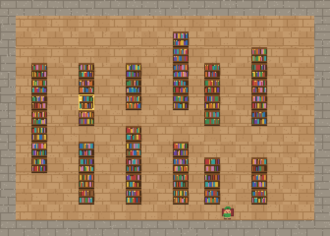
I was reading "Grokking Deep Reinforcement Learning" at the time, so the algorithms I picked came from the book, mainly model-free ones. Model-free means the agent doesn't know the rules of the environment in advance (no transition probabilities, no map of the obstacles, no reward function). What it does instead is visit a tile and think "I did this, I ended up here, I got this reward". It builds a value estimate purely from that stream of experiences. The algorithms differ almost entirely in one thing, how much of that stream to trust before updating anything.

Instead of just tracking a reward, I tracked how many steps above optimal a policy takes. Zero means it found the actual shortest path.

Every algorithm below explores the same way, with epsilon-greedy. Most of the time the agent takes the current best action it knows about, and with a small probability ε it picks one at random. That random pick is what I call a wander further down.

Monte Carlo

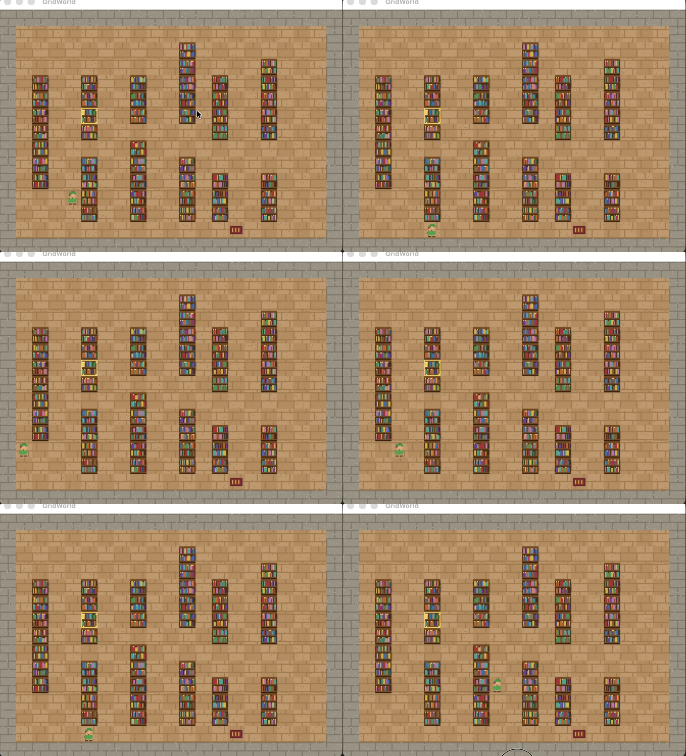
Monte Carlo (MC) methods estimate values by averaging the actual discounted return from complete episodes. One episode looks like this.

1. From the door, pick actions with epsilon-greedy, usually the current best, sometimes random. Walk until you find the book (or the episode is cut off). Store every (tile, action, reward) along the way.
2. Starting from the last step and walking backward, compute the actual discounted return that followed each visit, the rewards you really got from that point to the end of the episode.
3. Nudge Q(tile, action) a little toward that return, for every visit.
4. Repeat for the next episode. Nothing inside an episode gets corrected until the episode is over.

It's the slowest and noisiest method here. One unusually long or short episode swings every value visited along the way.

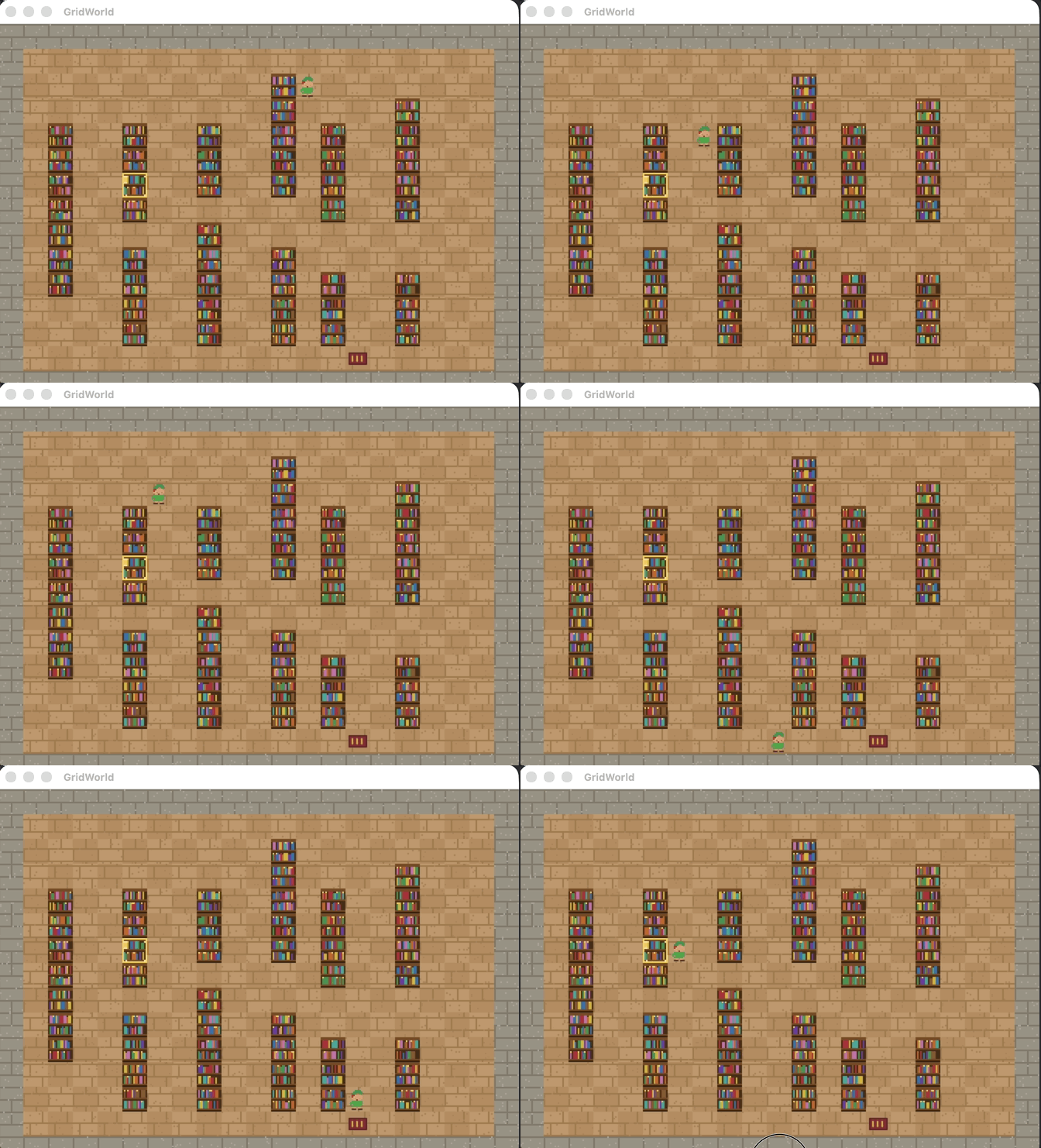
Here it is running in the library.

Bootstrapping

Monte Carlo waits until the book is found. Bootstrapping doesn't. After one step you look at the Q-value you already have for the next tile and treat that number as the rest of the return. Wrong at first, obviously, but you get an update on every move instead of once per episode.

SARSA, Expected SARSA and Q-learning all do that. They only disagree on which Q-value to borrow.

SARSA borrows the action it's actually about to take, wander included. It learns the value of its own messy, still-exploring behavior. That's on-policy.

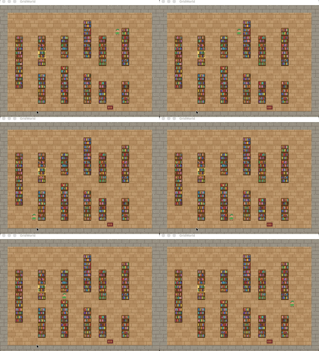
Expected SARSA still walks with epsilon-greedy, but the update averages every possible next action, weighted by how likely the policy is to pick it. Almost all the mass on the current best, a little on the wander. Same on-policy idea, without one unlucky random action swinging the target every step.

Q-learning always borrows the current best action from the new tile, even if you're about to wander. The walk can be messy. The update still pretends you'll be greedy next. That's off-policy, and it's why Q-learning is usually faster than SARSA. The values don't have to price in the chance that you'll slip.

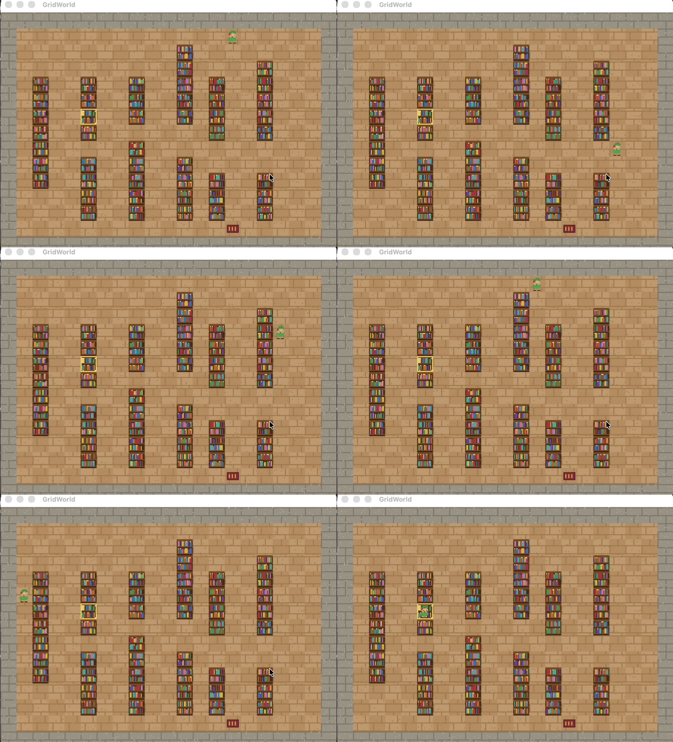
You don't have to bootstrap after exactly one step. n-step methods wait a few real rewards (I used 3) and then bootstrap. Same SARSA vs Q-learning split, just later. Eligibility traces drop the hard cutoff. Each step's error gets smeared across every recently visited (tile, action), decaying as you go. SARSA(λ) smears the on-policy error. Q(λ) smears the max, and if you wander it zeros the whole trace, because the trace was supposed to be a run of greedy actions and a random step breaks that.

I expected the extra real signal to help. On this library, with an epsilon that never decays, it mostly didn't.

Two tricks

Double Q-learning exists because max over noisy Q-values is biased, so plain Q-learning tends to get a bit too optimistic. Two tables. You pick actions from their sum. Each step a coin flip decides which table to update. Pick the best action according to the table you're updating, read that action's value from the other one. A noisy overestimate never gets to vouch for itself. On this task it behaved like regular Q-learning, just slightly more stable.

Dyna-Q is Q-learning plus a memory. Every real transition gets stored, then between actual steps it replays a batch of remembered ones as extra updates. The library is deterministic, so one memory per (tile, action) is the whole model. That's cheating in a useful way. More learning per real walk.