
Published April 7, 2026 · Revised July 24, 2026
Given observations from a discrete distribution, how much probability belongs to types you have not seen? The sample fingerprint – the counts of singletons, doubletons, and so on – supports a distribution-free estimator of that first quantity. It does not, by itself, identify how many unseen types exist or what their entropy contribution is; those questions require bounds, tail assumptions, or more data.
In the 1940s, the lepidopterist Alexander Corbet spent two years trapping butterflies in Malaya. He returned with a frequency table: 118 species observed exactly once, 74 observed twice, 44 three times, and so on. He brought the table to Ronald Fisher and asked: if I went back for another two years, how many new species would I find?
Fisher had to estimate a column of the table that didn’t exist: the zero column, the species Corbet never saw. Around the same time, at Bletchley Park, Alan Turing was working on the same problem in a different guise: estimating the probability of encountering a cipher pattern that had never appeared in intercepted traffic.
Both problems have the same structure: a finite sample from a fixed distribution whose support is unknown and possibly much larger than what you observed. The answer depends on the frequency of frequencies: how many species appeared exactly once, exactly twice, exactly three times, and so on. This vector is the fingerprint of the sample. It preserves what a label-invariant estimator can use, while discarding the species names.
# The fingerprint
Let be i.i.d. draws from a discrete distribution over an unknown support. Define:
The count is the number of singletons (species seen exactly once), and is the number of doubletons. The vector is the fingerprint.
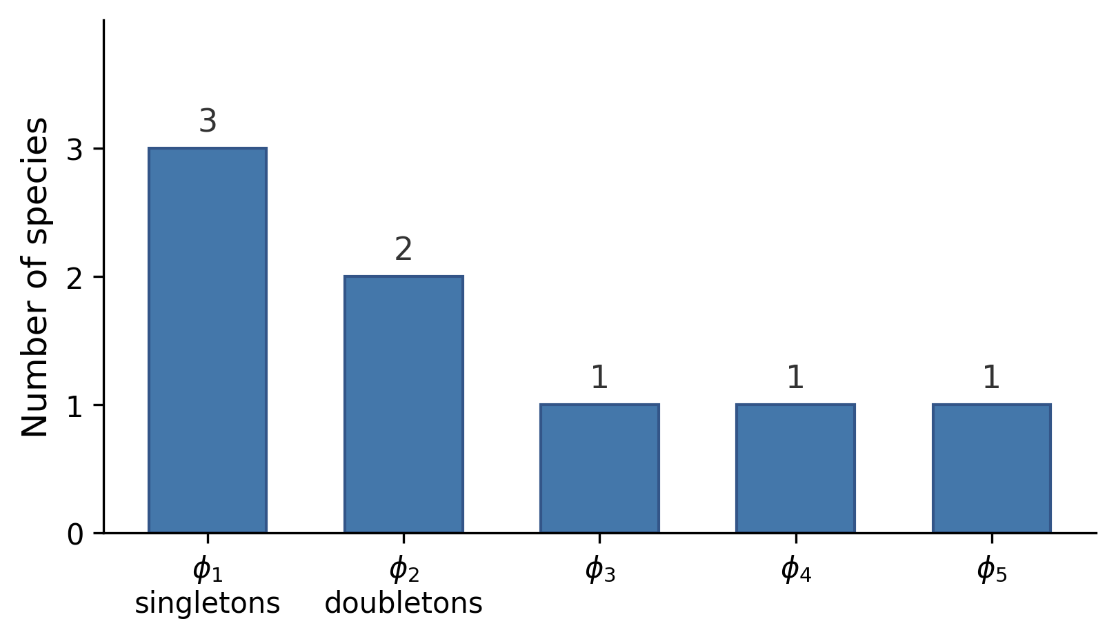
For a symmetric property, permuting the species labels does not change the target. Under a permutation-invariant loss, an estimator can therefore be symmetrized so that it depends only on the fingerprint, without worsening its worst-case risk.1 This is the useful invariance claim. It is not a universal privacy guarantee: a small or unusual fingerprint may itself disclose information, and non-symmetric questions still need the labels.
The singleton count is large when there are many rare species, species you barely caught. If is large relative to , you’ve probably missed a lot.
The code examples below use fingerprints, a Rust crate named after this data structure.
use fingerprints::Fingerprint;
let counts = [5usize, 4, 3, 2, 2, 1, 1, 1];
let fp = Fingerprint::from_counts(counts).unwrap();
assert_eq!(fp.sample_size(), 19);      // n = 5+4+3+2+2+1+1+1
assert_eq!(fp.observed_support(), 8);   // S_obs
assert_eq!(fp.singletons(), 3);         // phi_1
assert_eq!(fp.doubletons(), 2);         // phi_2
One fingerprint supports several questions, but they are not interchangeable:
| Question | Target | What extra structure controls the answer |
|---|---|---|
| How much probability is unseen now? | Missing mass | iid draws from one fixed distribution |
| How many new types will a larger sample discover? | Future discovery count | iid sampling plus a stated extrapolation horizon |
| How many types exist in total? | Support size | a lower-bound target, a support/tail model, or a sensitivity range |
| How uncertain is a draw? | Entropy | a known support regime, asymptotics, or an explicit prior model |
The next sections move through those targets in that order. A guarantee for one does not transfer to the next merely because all four can be estimated from the same fingerprint.
# Good-Turing: the probability of the unseen
Good (1953) gave an answer to “what fraction of the next observation will be a species we haven’t seen yet?”2
The missing mass (the total probability of all unseen species) is estimated by the fraction of singletons. If 3 of your 19 observations come from species seen only once, then roughly of the distribution’s probability mass belongs to species you never saw.
Why does this work? First Poissonize the total sample size: draw observations. Poisson splitting then makes the species counts independent, with
For species ,
The random missing mass is , while . Taking expectations gives
This is the complete Poissonized identity: a zero-count probability on one side becomes a singleton probability on the other. With exactly independent draws, the two expectations are close but not identical:
The remaining bias is at most order . Distribution-free concentration results control the random error uniformly over the choice of , but “distribution-free” does not mean assumption-free: the observations must still be independent draws from one fixed distribution.If the population drifts while you sample, mixes novelty with drift. No iid missing-mass theorem repairs that change of data-generating process.
The complementary quantity is sample coverage: . Coverage of 84% means the observed species account for 84% of draws from the underlying distribution.
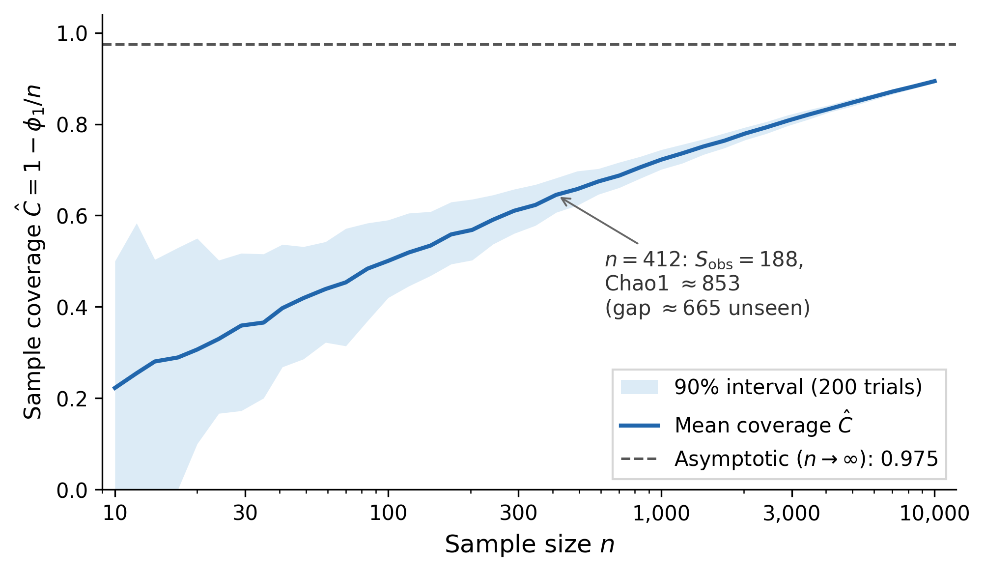
More generally, Good-Turing smoothing reassigns probabilities to every frequency class: a species seen times gets estimated probability where .17This has a pathology at : the most frequent species gets probability zero because . Gale and Sampson (1995) fix this with log-linear smoothing of the frequency spectrum. The missing mass formula is the special case .
There is a fundamental limit on species-count extrapolation. Orlitsky, Suresh, and Wu (2016) proved that predicting how many new species appear in future samples works when , but beyond that horizon no estimator is consistent.18 This result is about forecasting new-species counts, not about the missing mass estimator itself: for missing mass, the minimax risk is with no phase transition.Rajaraman, Thangaraj, and Suresh (2017, arXiv:1705.05006) establish the minimax lower bound for missing mass estimation, showing risk and no analogue of the log n threshold.
Good formalized and published Turing’s wartime work in 1953.2 The same smoothing problem became central to statistical language modeling. Chen and Goodman’s 1998 survey16 compares Good-Turing discounting with backoff and interpolation methods, including Katz and Kneser–Ney.
A historical validation came from Efron and Thisted’s 1976 Shakespeare vocabulary study. They used the fingerprint of word frequencies in the known canon to predict how many new words would appear if an additional text were discovered.Shakespeare’s known works contain 31,534 distinct word types across roughly 884,000 tokens. Of those, 14,376 appear exactly once – hapax legomena. That alone is 46% of the vocabulary. When an unknown poem attributed to “W.S.” surfaced in the Bodleian Library in 1985, their model predicted new words. The actual count was 9. They also tested poems by Jonson, Marlowe, and Donne against the Shakespearean fingerprint; all failed.10
# A full-fingerprint correction
Good-Turing uses only . Lee and Böhme propose an alternating full-fingerprint correction:22
The first term is Good-Turing. Under their fixed-distribution sampling model, the later terms cancel its finite-sample bias more aggressively. That is a bias statement, not a dominance theorem: the alternating estimator can have higher variance, especially for skewed distributions, so mean-squared error can still favor the singleton estimate.
# How many species total?
# Chao1: estimating a lower-bound target
Chao (1984) gave a lower bound on the total number of species :3
The lower bound comes from one Cauchy–Schwarz step. In the Poissonized model, let and write . The expected numbers of unseen, singleton, and doubleton species are
Applying Cauchy–Schwarz to the sequences and gives
Because total support is observed species plus unseen species,
This is a lower bound expressed through expected frequency counts. Replacing those expectations with the observed and gives an estimator of that lower-bound target. The realized estimate is not guaranteed to lie below , nor is its finite-sample expectation always below .
The smallest counterexample needs only two equiprobable species and three draws. With probability , all draws match and Chao1 returns 1. Otherwise the counts are and it returns . Its expectation is therefore , above the true support of 2:
from itertools import product
def chao1(sample):
    counts = [sample.count(0), sample.count(1)]
    f1 = sum(count == 1 for count in counts)
    f2 = sum(count == 2 for count in counts)
    observed = sum(count > 0 for count in counts)
    return observed + (f1 * f1 / (2 * f2) if f2 else f1 * (f1 - 1) / 2)
print(sum(chao1(list(sample)) for sample in product(range(2), repeat=3)) / 8)
# 2.125
The lower-bound interpretation remains useful: heterogeneous rare-species probabilities generally leave Chao1 below the total richness it is meant to estimate. It should be reported as a richness estimator derived from a lower bound, not as a one-sided finite-sample guarantee.
The term estimates the unseen count from the ratio of singletons to doubletons. If you have many singletons but few doubletons, the singletons look like the tip of an iceberg.When , the formula divides by zero. Software implementations use the bias-corrected fallback . Zero doubletons occur routinely in small samples from skewed distributions.
use fingerprints::{Fingerprint, support_chao1, support_chao1_with_ci};
let fp = Fingerprint::from_counts([5, 3, 2, 1, 1]).unwrap();
let s_hat = support_chao1(&fp);
assert!(s_hat >= fp.observed_support() as f64);
// With estimated variance and an approximate 95% interval:
let est = support_chao1_with_ci(&fp);
println!("[{:.1}, {:.1}, {:.1}]", est.ci_lower, est.point, est.ci_upper);
The log-transformed interval is an asymptotic uncertainty approximation. It is not a certificate that contains the true richness 95% of the time for every finite distribution.
A cautionary note: Chao1 is available as an alpha-diversity metric in microbiome tools like QIIME2 and mothur, but ASV-based denoising pipelines collapse rare variants, destroying the singleton count that Chao1 depends on. Deng, Umbach, and Neufeld (2024) warned that Chao1 “must not be used” with ASV data13, a case where preprocessing violates the estimator’s assumption. If your pipeline collapses rare types before counting, and no longer mean what Chao1 thinks they mean.
# iChao1: pulling in higher frequencies
Chiu, Wang, Walther, and Chao (2014) improved the lower bound using (tripletons) and (quadrupletons):4
When , the displayed correction is undefined; the fingerprints implementation falls back to Chao1. When , the correction is zero. Otherwise iChao1 is at least as large as Chao1 and uses more of the fingerprint. The correction term captures information about the tail that and alone miss.
# A linear-program sensitivity range
Valiant and Valiant showed how to estimate the unseen shape of a distribution, and hence symmetric properties such as support size and entropy, at optimal sample-complexity rates.5 The first result appeared at STOC 2011; the improved estimator appeared at NeurIPS 2013, not STOC 2013.
The local fingerprints crate contains a smaller VV-style research scaffold. It places the unknown probability histogram on a finite log-spaced grid, asks that its Poisson-expected fingerprint match the observed one within configurable tolerances, and minimizes or maximizes a property over the feasible set. Its endpoints depend on the grid, probability cutoff, and tolerance. They are sensitivity ranges for that discretized model, not distribution-free confidence intervals and not a reimplementation of the full VV theorem.
The following example shows how wide the feasible range can be from 19 observations; its width quantifies sensitivity to this particular grid and tolerance policy:
use fingerprints::{Fingerprint, to_bits};
use fingerprints::vv::{support_bounds_lp, entropy_bounds_lp, LpParams};
let fp = Fingerprint::from_counts([5, 4, 3, 2, 2, 1, 1, 1]).unwrap();
let params = LpParams::default_for(&fp);
let (s_lo, s_hi) = support_bounds_lp(&fp, params.clone()).unwrap();
println!("grid-feasible support range: [{:.0}, {:.0}]", s_lo, s_hi);
let (h_lo, h_hi) = entropy_bounds_lp(&fp, params).unwrap();
println!("grid-feasible entropy range: [{:.2}, {:.2}] bits",
    to_bits(h_lo), to_bits(h_hi));
Run cargo run --example vv_bounds in the fingerprints repository to reproduce the calculation. Change grid_size, p_min, and eps_scale before treating either endpoint as stable.
# Entropy in the unseen regime
Estimating Shannon entropy from a finite sample is biased. The naive plug-in estimator systematically underestimates because it misses unseen species entirely.
The first three estimators below are frequentist corrections to the empirical entropy and are most interpretable in a fixed or effectively bounded support regime. The minimax results later in the section assume a known or bounded alphabet size. Pitman–Yor instead opens a model-based branch for countably infinite, heavy-tailed alphabets. These are different assumption sets, not successive rungs of one universally improving ladder.
Four estimators illustrate the resulting approaches.
# 1. Plug-in (maximum likelihood)
Negatively biased. It becomes useful when the empirically relevant support is well sampled; is a finite-support rule of thumb, not a universal threshold for heavy or countably infinite tails.
# 2. Miller-Madow
A first-order bias correction due to Miller (1955).6 When (many singletons), the correction can overshoot.
# 3. Jackknife
Under smooth, fixed-effective-support asymptotics, delete-one jackknifing removes the leading bias term, leaving an term.7 Large or countably infinite supports need additional conditions and empirical calibration:
Computed efficiently from the fingerprint without enumerating all leave-one-out samples.
These three estimators do not exhaust the field. Jiao, Venkat, Han, and Weissman (2015) and Wu and Yang (2016) showed that polynomial-approximation estimators attain the minimax entropy rate when the alphabet size is known or bounded; consistent estimation begins around samples.19 Hao and Orlitsky (2019) gave a near-linear-time profile-likelihood method with sample-optimal guarantees for a broad class of additive symmetric properties under their regularity conditions.20 Those guarantees are property- and regime-specific, not a license to call every fingerprint-derived estimate optimal.
# 4. Pitman-Yor
Archer, Park, and Pillow developed Bayesian entropy estimators for countably infinite alphabets and showed why power-law priors can help in undersampled regimes.8 The Pitman-Yor process has discount and concentration . For , its expected number of occupied types grows polynomially rather than logarithmically as in the Dirichlet-process case.
The estimator in fingerprints is a different, newer construction: it implements the predictive-distribution method of Hashino and Tsukuda (2026) and selects by minimizing their plug-in cross-entropy bound.23 That implementation should be evaluated against the distributions and sample sizes where it will be used. The prior’s ability to express a power-law tail does not guarantee lower finite-sample error than a classical correction.
use fingerprints::{Fingerprint, entropy_pitman_yor_nats, pitman_yor_params_hat, to_bits};
let fp = Fingerprint::from_counts([5, 4, 3, 2, 2, 1, 1, 1]).unwrap();
let h_py = entropy_pitman_yor_nats(&fp);
let py = pitman_yor_params_hat(&fp);
println!("H = {:.3} bits  (d={:.3}, alpha={:.3})",
    to_bits(h_py), py.d, py.alpha);
# A replicated example
One simulation trajectory can make any estimator look unusually good or bad. The figure below uses 400 independent trials at each sample size from a finite Zipf$(1.1)$ distribution over 5,000 types. The true entropy, computed directly from that normalized distribution, is 7.914183 bits.
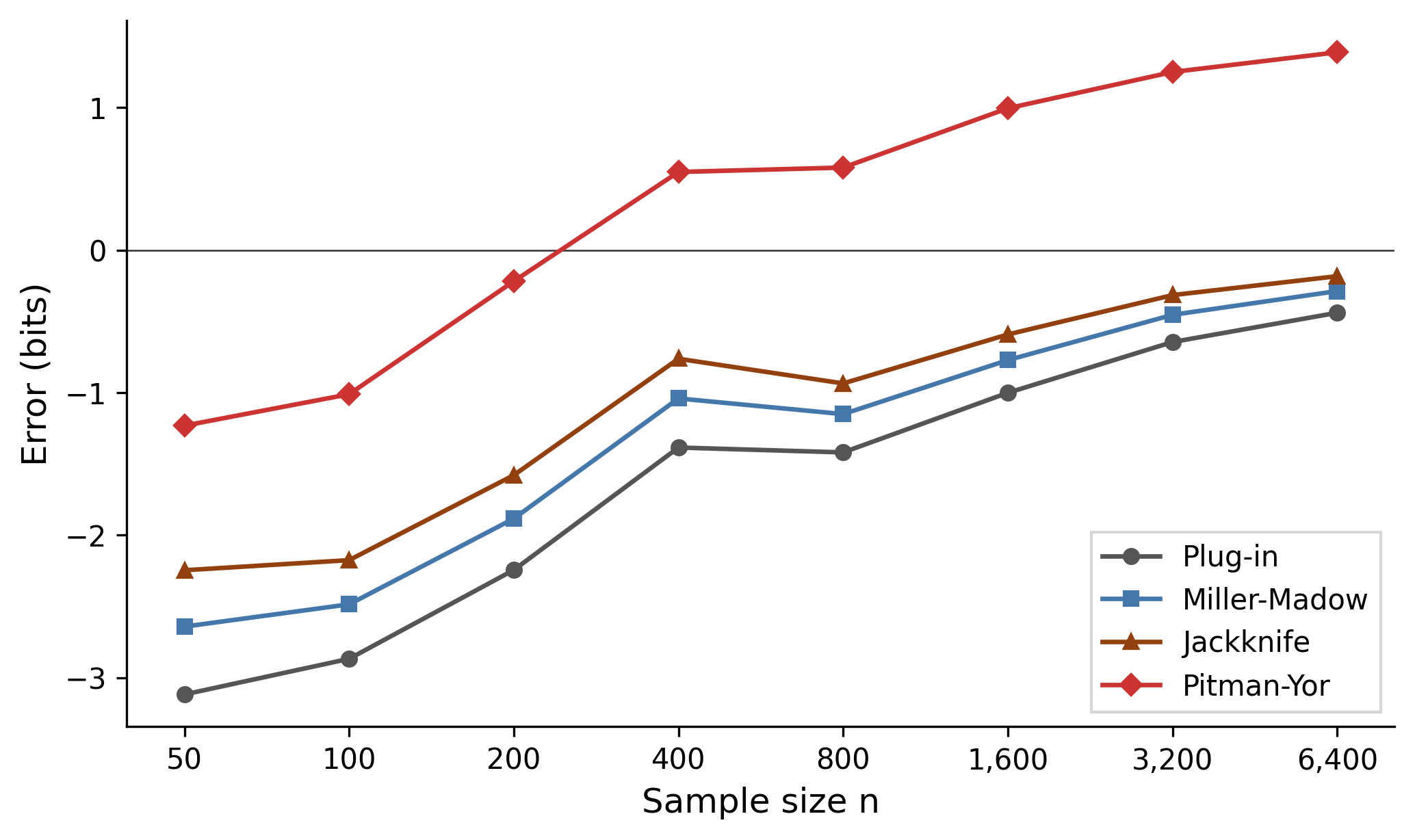
At , the mean errors are bits for plug-in, for Miller–Madow, and for jackknife. At , they are , , and bits. Those numbers describe this finite Zipf experiment, not a universal ordering. The generator reports both mean error and root-mean-square error at every point.
The Pitman-Yor implementation is not part of this comparison. Evaluating it fairly requires running the specified Rust implementation, including its parameter-selection policy, inside every replicate. Results from a different implementation do not establish its convergence behavior.
# When estimators disagree
Different estimators make different assumptions about the tail. Their spread is useful as a sensitivity diagnostic: it shows how much the answer moves when the modeling choice changes. It is not a confidence interval. Three wrong estimators can agree, and three noisy estimators can disagree even when one is well calibrated.
| Question | What the result means |
|---|---|
| Unseen probability mass | Good-Turing estimates it under iid sampling from one fixed distribution |
| Conservative richness target | Chao1 or iChao1 estimate a lower-bound target; neither is a finite-sample one-sided guarantee |
| Entropy with a known support bound | Polynomial-approximation methods have minimax guarantees in specified regimes |
| Entropy under a power-law model | A Pitman-Yor method is a model-based estimate whose calibration should be simulated |
| Local LP range | The fingerprints VV-style scaffold measures sensitivity to its grid and tolerances |
Report the estimand, assumptions, and a sampling uncertainty calculation that matches the estimator. Reporting several point estimates can supplement that work; it cannot replace it.
Two applications make the stakes concrete. In forensic DNA, when a suspect’s DNA profile matches a crime scene sample but has never appeared in the reference database, empirical frequency estimation gives a match probability of zero. That zero reflects the estimator rather than evidence that the profile is impossible. This is the missing mass problem directly: “what is the probability of a type we haven’t seen?” Favaro and Naulet (2023) frame it as a Good-Turing problem and prove optimal bounds.12
In software fuzzing, Böhme (2018) mapped the framework onto security testing: execution paths are species, fuzzer runs are samples. Good-Turing estimates the probability that another run discovers a path not yet observed.14 If estimates disagree, the current fingerprint does not support a model-insensitive answer. More fuzzing may narrow the gap, but only if future executions are comparable draws from the same path-generating process.
# The fingerprint everywhere
The same structure recurs far beyond ecology.
Your immune system contains distinct T-cell receptor clonotypes generated by VDJ recombination, but any blood draw captures a tiny fraction. Each clonotype is a species, each sequenced cell is a sample. Laydon et al. (2015) showed that classical estimators severely undercount because the TCR frequency distribution is heavy-tailed.11 An unusually diverse repertoire correlates with effective viral control, and the unseen fraction has direct clinical relevance for HIV, cancer immunotherapy, and aging.
At the other end of the scale, HyperLogLog (Flajolet et al., 2007) estimates the number of distinct elements in a data stream, a related support-size question solved with hash-based sketches rather than an observed fingerprint.The distinction matters: ordinary HyperLogLog does not retain the sample’s frequency-of-frequencies vector. Cohen (2016) developed extensions that estimate richer frequency statistics from sketches. Implementations appear in Redis, Spark, and PostgreSQL via an extension.15
The German tank problem is a useful contrast. Consecutive serial numbers justify a uniform-with-unknown-endpoint model and the estimator , where is the largest observed serial and is the sample size. Species labels carry no such ordering. The broad question is similar, but the extra structure changes the mathematics.
The fingerprint links applications from cryptanalysis and microbiome sequencing to forensic evidence and database cardinality. Each asks what remains unseen after incomplete sampling.
# References
[1] Acharya, Das, Orlitsky, Suresh, “A unified maximum likelihood approach for estimating symmetric properties of discrete distributions,” ICML 2017. ↩
[2] I.J. Good, “The population frequencies of species and the estimation of population parameters,” Biometrika 40(3/4), 237–264, 1953. The core idea is due to Turing; Good credits him explicitly but is the sole listed author. ↩
[3] Anne Chao, “Nonparametric estimation of the number of classes in a population,” Scandinavian Journal of Statistics 11(4), 265–270, 1984. ↩
[4] Chiu, Wang, Walther, Chao, “An improved nonparametric lower bound of species richness via a modified Good-Turing frequency formula,” Biometrics 70(3), 671–682, 2014. ↩
[5] Gregory Valiant, Paul Valiant, “Estimating the unseen: An -sample estimator for entropy and support size, shown optimal via new CLTs,” STOC, 685–694, 2011. Journal version: JACM 64(6), 2017. Follow-up: Paul Valiant and Gregory Valiant, “Estimating the Unseen: Improved Estimators for Entropy and other Properties,” NeurIPS 2013, 2157–2165. ↩
[6] G.A. Miller, “Note on the bias of information estimates,” in Information Theory in Psychology, Free Press, 95–100, 1955. Often called “Miller-Madow” by convention, though Madow is not a co-author. ↩
[7] S. Zahl, “Jackknifing an index of diversity,” Ecology 58(4), 907–913, 1977. ↩
[8] Evan Archer, Il Memming Park, Jonathan W. Pillow, “Bayesian entropy estimation for countable discrete distributions,” JMLR 15, 2833–2868, 2014. Conference version: NeurIPS 2012. ↩
[10] Bradley Efron, Ronald Thisted, “Estimating the number of unseen species: How many words did Shakespeare know?”, Biometrika 63(3), 435–447, 1976. The validation: Thisted and Efron, “Did Shakespeare write a newly-discovered poem?”, Biometrika 74(3), 445–455, 1987. ↩
[11] Laydon, Bangham, et al., “Estimating T-cell repertoire diversity: limitations of classical estimators and a new approach,” Phil. Trans. R. Soc. B 370, 20140291, 2015. ↩
[12] Favaro, Naulet, “Optimal estimation of high-order missing masses, and the rare-type match problem,” arXiv:2306.14998, 2023. ↩
[13] Deng, Umbach, Neufeld, “Nonparametric richness estimators Chao1 and ACE must not be used with amplicon sequence variant data,” The ISME Journal, 2024. ↩
[14] Marcel Böhme, “STADS: Software Testing as Species Discovery,” ACM TOSEM 27(2), 2018. ↩
[15] Flajolet, Fusy, Gandouet, Meunier, “HyperLogLog: the analysis of a near-optimal cardinality estimation algorithm,” AofA, 2007. Cohen, “HyperLogLog Hyper Extended,” arXiv:1607.06517, 2016. ↩
[16] Chen, S. F. & Goodman, J. (1998). “An empirical study of smoothing techniques for language modeling.” Technical Report TR-10-98, Harvard University. ↩
[17] Gale, W. A. & Sampson, G. (1995). “Good-Turing frequency estimation without tears.” Journal of Quantitative Linguistics, 2(3), 217–237. ↩
[18] Orlitsky, A., Suresh, A. T. & Wu, Y. (2016). “Optimal prediction of the number of unseen species.” Proceedings of the National Academy of Sciences, 113(47), 13283–13288. ↩
[19] Jiao, J., Venkat, K., Han, Y. & Weissman, T. (2015). “Minimax estimation of functionals of discrete distributions.” IEEE Transactions on Information Theory, 61(5), 2835–2885. arXiv:1406.6956. Wu & Yang (2016, arXiv:1407.0381) give tight constants for entropy. ↩
[20] Hao, Y. & Orlitsky, A. (2019). “The Broad Optimality of Profile Maximum Likelihood.” NeurIPS 2019. ↩
[22] Lee, S. & Böhme, M. (2025). “How Much is Unseen Depends Chiefly on Information About the Seen.” ICLR 2025. ↩
[23] Hashino, T. & Tsukuda, K. (2026). “Estimating the Shannon Entropy Using the Pitman–Yor Process.” arXiv:2602.08347. ↩
← Regions for Set Inclusion
Comments
Nothing yet. Say the first thing.
Sign in to join the conversation.