A Difference Table Is a Discrete Derivative

Published December 10, 2024 · Revised July 24, 2026

Subtract consecutive terms of a sequence, then repeat. For a polynomial sequence, each pass removes one degree until only a constant remains. When the sequence counts genuinely nested stages, the first differences have an even more literal meaning: they count the points added in each new layer. Without nesting, they record only net change.

Start with the triangular numbers:

Subtract each term from the next. Then do the same to the new row.

Reproduce this figure

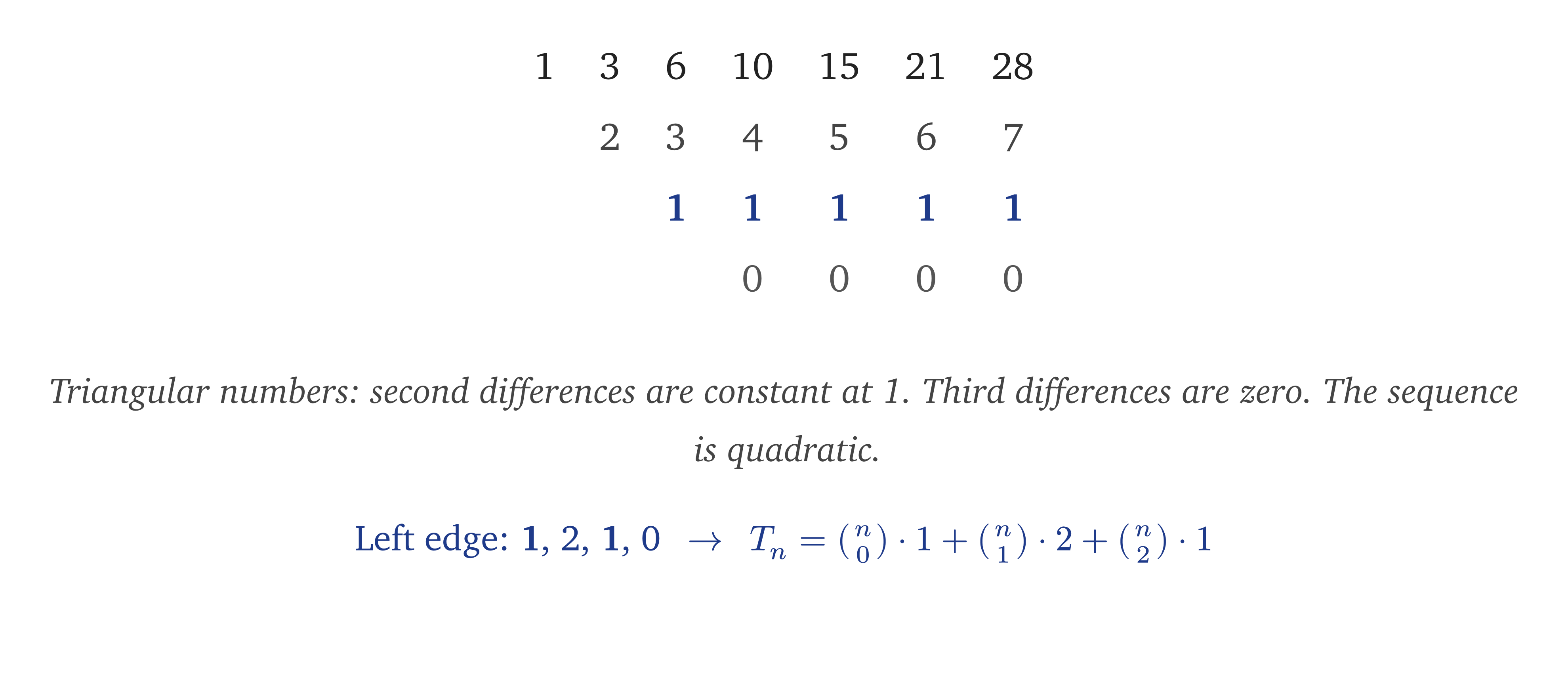
The first row says how much the triangles grow: add 2 dots, then 3, then 4. The next row says that those additions themselves grow by 1 each time. After one more subtraction, nothing changes.

That calculation introduces the main ideas used below.

# A map of the argument

There are three directions to follow:

1. Down the table: differences remove polynomial degree, while nonpolynomial signatures leave periodic, exponential, or recursive structure behind.
2. From objects to numbers: geometric stages become totals and changes. Equal totals can forget the shape, while different weights retain or isolate different information.
3. Back up the table: summation stacks the layers, while the left edge reconstructs the sequence. The Stirling-number coefficients explain the special case of ordinary powers.

The final section explains why exact and measured sequences behave so differently under repeated differencing.

One pattern connects the geometric examples: start with a filtered family of objects, measure each stage, and then take a discrete derivative. A valuation is such a measurement when it respects inclusion–exclusion: . Cardinality, ordinary volume, and sums of fixed point weights are examples in the settings below. The difference table belongs to the resulting numbers; whether those differences still describe literal layers depends on what the valuation forgot.

# Differences peel off degree

For a sequence given by a function , define its forward difference by

If is a degree- polynomial, then has degree . For example, if the leading term is , the binomial theorem gives

Repeat this times and only the constant remains. One more difference gives zero. Thus:

• a linear sequence has constant first differences;
• a quadratic sequence has constant second differences;
• a cubic sequence has constant third differences.

The cubes make the last case visible.

Reproduce this figure

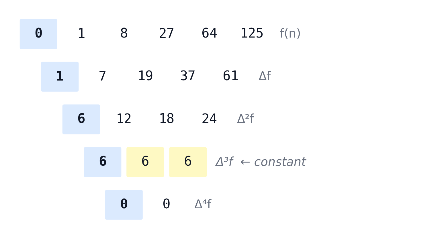
This works in reverse. If an infinite sequence has zero $(d+1)$st differences everywhere, it comes from a polynomial of degree at most . A short finite table can always be fitted by a polynomial, so the test becomes conclusive only when the pattern is known to continue.

The arithmetic needs only a few lines:

def difference_table(values):
    rows = [list(values)]
    while len(rows[-1]) > 1:
        previous = rows[-1]
        rows.append([b - a for a, b in zip(previous, previous[1:])])
    return rows

Finite differences also obey a product rule, but the shift cannot be omitted:

Equivalently, the shift may fall on instead. This small asymmetry is one way that finite differencing departs from ordinary differentiation. The coordinates adapted to this operator will appear when the article rebuilds a sequence from its left edge.

# When a difference is a new layer

Suppose is the set of points present at stage , and let . Passing from the objects to their counts, then to their differences, gives a one-way flow:

Each arrow forgets something. The total forgets where the points are. The difference forgets which points arrived and which departed.

If the stages are nested,

then nothing departs. The new shell at stage is

and its size is exactly

That set identity – not the sequence alone – is what makes a difference into a new layer.

Now put points on a triangular grid. From any point, allow one step in any of the six grid directions. The points reachable in at most steps form a hexagon.

Reproduce this figure

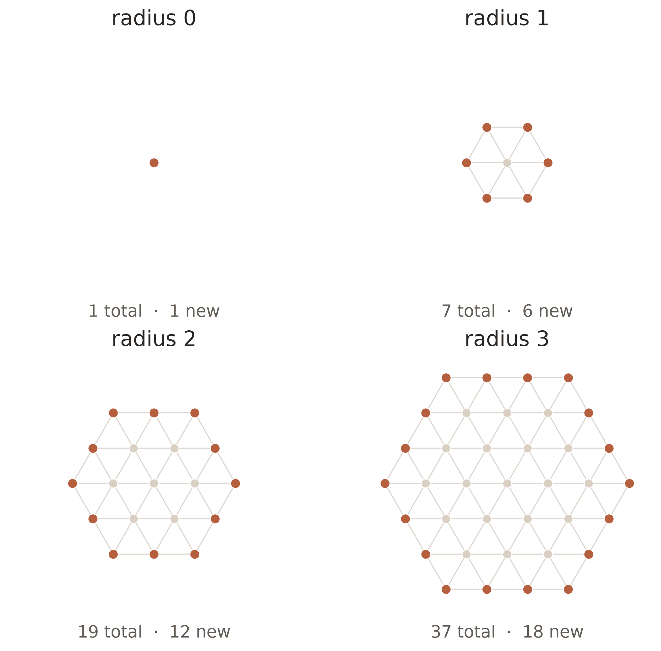
At radius , the total number of points is

So the ring added at radius has

points. The six sides each gain one point per unit of radius. The geometric layers and the rows of the difference table are the same count:

radius	total	new ring
0	1	1
1	7	6
2	19	12
3	37	18

Reproduce the lattice counts

generator lockfile uv run --locked hexagonal_growth.py

The totals are quadratic, the rings are linear, and the change in ring size is the constant 6.

The same hexagon is the ball of radius for the six allowed moves on the root lattice.1 Changing the allowed moves changes the ball and can change the sequence.

# Net growth is not always a shell

The nesting condition is a separate requirement. Consider the interval on the integer line. Its $n$th dilation contains

so its count is always . From to , however, the set changes from

Two points, 5 and 6, arrive; one point, 2, disappears. The count rises by one, but there is no one-point shell. The first difference records arrivals minus departures.

For a convex shape , putting the origin inside is a sufficient condition for nested dilations:

That is why the centered hexagons above form nested set-theoretic layers while an arbitrary translation of the same counting problem may not.

# The polygon formula

There is a wider two-dimensional rule. Let be a polygon whose vertices lie on the integer lattice. If is its area and is the number of lattice points on its boundary, then the number of lattice points in its -fold dilation is

This is the polygon case of Ehrhart counting, and it follows directly from Pick’s theorem.2 One difference turns that quadratic total into a linear net increment. When the dilations are nested, that increment is the size of the new set. For the hexagon above, and , so and the $n$th layer has exactly points.

A new layer need not equal the geometric boundary for every polygon. It does for this centered hexagon: the strictly interior lattice points of the $n$th hexagon are exactly the points already present at radius . The distinction matters when the shape is changed.

# The table forgets the shape

The same count can come from a different picture. Compare the unit square

with the stretched triangle

The $n$th dilation of the square has lattice points. The triangle has rows of lengths

whose sum is also

The two shapes therefore have the same sequence and the same difference table for every nonnegative integer dilation. They are Ehrhart-equivalent. This is a useful limit on what a table can reveal: it records the counting function, not a unique geometry.

The equality is not a numerical accident. Both polygons have area 1, four boundary lattice points, and no interior lattice points, so the polygon formula gives for each. Their shapes and their corresponding counting arguments remain different.

Equal totals at every scale are therefore weaker than equal point sets, equal layers, or a geometric map between the shapes. A plain difference table cannot distinguish those notions because it receives only one number per stage.

# Keep one coordinate and the collision disappears

The input can retain more information. Instead of giving every lattice point weight 1, retain its horizontal coordinate:

At scale one, the square gives

while the stretched triangle gives

Their ordinary counts agree because both expressions become 4 at . Before that substitution, the weighted counts remember enough horizontal position to tell the shapes apart. A two-variable sum

records the entire finite lattice-point set at that scale. It still does not turn one sampled scale into the continuous polygon, but it makes the information tradeoff explicit. Weighted Ehrhart theory develops this idea systematically.5

There are other ways to ask a richer family of questions. For example, the Ehrhart quasipolynomials of all rational translations of a rational polytope determine it up to an integer translation.6 One count is coarse; a carefully chosen profile can distinguish much more.

# Changing the weight changes the question

Coordinate weights preserve more location. A different weighting can instead remove a feature that the ordinary count mixes in.

For a positive dilation of a lattice polygon, give an interior lattice point weight 1, a nonvertex point on an edge weight , and a vertex the fraction of a full turn occupied by the polygon’s interior angle. The sum of these solid-angle weights is

In the unit square, for example, has interior points, nonvertex edge points, and four right-angle vertices. The weighted sum is

The ordinary count is ; the solid-angle count is . The first includes the boundary correction and the universal stage-zero point. The second isolates area. Neither is the uniquely correct count: each answers a different question. Macdonald’s solid-angle analogue of Ehrhart counting places this calculation in a general valuation theory.7

# Summation stacks the layers

Differencing removes a layer. Summation puts the layers back.

The square-pyramidal numbers make this literal:

They count stacks whose horizontal layers contain points. Therefore

The same argument works for a height-one lattice pyramid over any lattice polytope . Its integer-height slices are copies of , in reverse order, so

Taking one forward difference recovers the next slice:

Sam and Woods use this slice-and-sum idea as the elementary core of a proof of Ehrhart’s theorem.3 The general proof is more careful, but the picture already explains why summing raises polynomial degree by one and differencing lowers it by one.

# The left edge keeps the sequence

A difference table does not only reveal the degree. Its left edge rebuilds the sequence.

Let shift a sequence forward, so . The definition of a forward difference says

Advancing from to applies the shift times. Because and commute, the ordinary binomial theorem gives

This is Newton’s forward formula.4 The formula is therefore a finite operator identity at each integer , not a convergence claim and not a test that the sequence is polynomial. What is special about a degree- polynomial is that the expansion terminates globally: for every , so the upper limit can be replaced by for every .

The basis in that formula is not arbitrary. Pascal’s identity gives

The binomial polynomials lower one index at a time under differencing, just as ordinary powers lower degree under differentiation. That lowering property is why the left-edge values are their coefficients.

For the triangular sequence as indexed in the opening, the left edge is . Therefore

The apparent shift is only indexing: is the first triangular number, not the zeroth. For a general sequence, the same identity still reconstructs each term, but the number of left-edge coefficients needed grows with .

# Why the cube table contains 1, 6, 6

The left edge of the cube table is

Those numbers are not specific to cubes. For the sequence ,

where is a Stirling number of the second kind: the number of ways to partition an -element set into nonempty blocks.

The alternating sum has a direct counting meaning. There are functions from an -element set to labeled targets. Inclusion-exclusion removes the functions that miss one or more targets, leaving the surjections onto targets. An unordered partition into blocks becomes a surjection after the blocks are assigned to the target labels, which can be done in ways.

For ,

Multiplying by gives . Newton’s formula then reads

This is the change of basis hiding in the difference table: ordinary powers are being rewritten in binomial polynomials, and Stirling numbers are the conversion coefficients.

# Tables that do not flatten

Polynomial tables eventually reach zero. Other sequences leave different signatures.

# A polynomial with a clock

Integer polytopes give polynomial counts. Rational polytopes generally give quasipolynomials: each residue class follows a polynomial, but the formulas can differ periodically.

The interval

already shows the effect. Its $n$th dilation contains

integer points, so the totals begin

and the first differences alternate

The linear trend has been removed, but the period-two clock remains. Higher differences keep oscillating instead of becoming zero. A nonflattening table can therefore mean “polynomial growth plus a periodic residue,” not only exponential or recursive growth.

# Exponential and recursive signatures

For ,

so every row of the table repeats the same powers of two, shifted and shortened. More generally, is an eigenfunction of the difference operator:

The Fibonacci numbers have a different pattern.

Reproduce this figure

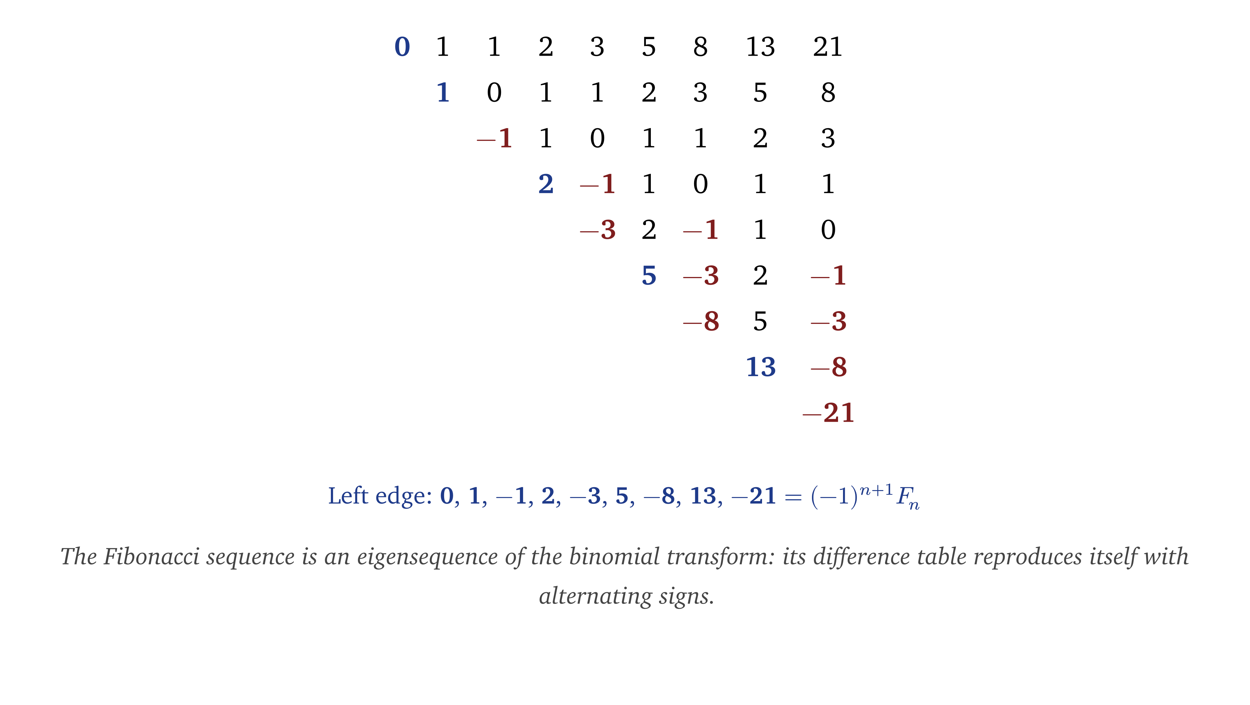
Reading down the left edge applies the signed binomial transform

For Fibonacci,

One quick explanation comes from Binet’s formula. Differencing sends an exponential to at the row level, and sends its left-edge transform to . The two Fibonacci roots satisfy and , so the roots exchange places and pick up alternating signs.

The table never becomes constant because Fibonacci is not polynomial, but it still exposes the algebra governing the sequence.

# Exact sequences and noisy measurements

Everything above uses exact values. A difference table is much less forgiving when the entries contain measurement or rounding error.

Suppose an otherwise smooth sequence contains a small alternating error . One difference turns it into

After rows, its magnitude is . The highest-frequency error doubles at every step even while differencing removes the smooth polynomial trend.

Random error has a related but distinct amplification law. If the observation errors are independent, have mean zero, and share variance , then

Independence removes the cross terms in the variance, so

Thus the standard deviation grows by , asymptotically close to . The exact gain above belongs to a deterministic alternating mode. If errors are correlated, the variance is instead , where ; the independence formula must not be reused unchanged.

For an exact sequence with a difference law known to continue, a constant row settles the polynomial question. With measured data, high-order differences are a diagnostic, not proof of a polynomial law; smoothing, uncertainty, and out-of-sample checks matter.

# What the table is saying

A first difference is the net change at the next step. It becomes the amount added only when the underlying stages are nested. Repeated differences measure how that growth itself changes. For polynomial sequences, the process ends after finitely many rows, and the left edge records the coefficients in the binomial basis.

In geometric counting, the flow of information matters. A filtered family of objects is measured by a valuation; differencing then takes the discrete derivative of that measurement. Weighted counts retain selected structure that a plain total discards. When the sets form a filtration, totals become layers, layers become changes in the boundary, and a pyramid is a running sum of its slices. The table is not only a way to guess a formula. Read with its assumptions visible, it is a record of how the object grows – and of what was forgotten in turning that object into a sequence.

Verify the article's exact identities

verification program uv run verify_identities.py --max-n 6

# References

[1] Ardila, F., Beck, M., Hoşten, S., Pfeifle, J., and Seashore, K. “Root Polytopes and Growth Series of Root Lattices.” SIAM Journal on Discrete Mathematics 25(1):360–378, 2011. ↩

[2] Beck, M. and Robins, S. Computing the Continuous Discretely. Springer, 2007. Chapters 2 and 3 cover Pick’s theorem and Ehrhart counting. ↩

[3] Sam, S. V. and Woods, K. M. “A Finite Calculus Approach to Ehrhart Polynomials.” The Electronic Journal of Combinatorics 17, R68, 2010. ↩

[4] Graham, R. L., Knuth, D. E., and Patashnik, O. Concrete Mathematics: A Foundation for Computer Science. 2nd ed., Addison-Wesley, 1994. Chapter 2 develops finite differences, falling factorials, and Newton’s formula. ↩

[5] De Loera, J. A., Valencia, C. E., Villarreal, R. H., and Wang, C. “Ehrhart Functions of Weighted Lattice Points.” arXiv:2412.17679. ↩

[6] Higashitani, A., Murai, S., and Yoshinaga, M. “Ehrhart Quasi-polynomials and Parallel Translations.” arXiv:2307.08151. ↩

[7] Beck, M. and Ehrenborg, R. “Ehrhart-Macdonald Reciprocity Extended.” Moscow Mathematical Journal 5(3):495–504, 2005. ↩

← Passive WiFi Channel Hopping as Active Sensing Why 561 Passes Fermat's Test →