The Training Inspect System

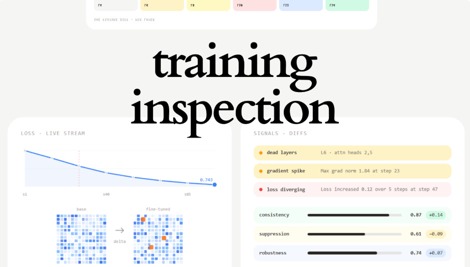
A fine-tuning run has structure beneath the loss curve: gradient dynamics that reveal how information flows through the network, attention heads that can collapse silently, feature activations that shift as the model rewrites internal representations to accommodate the training objective. Almost none of that structure is visible from loss alone.

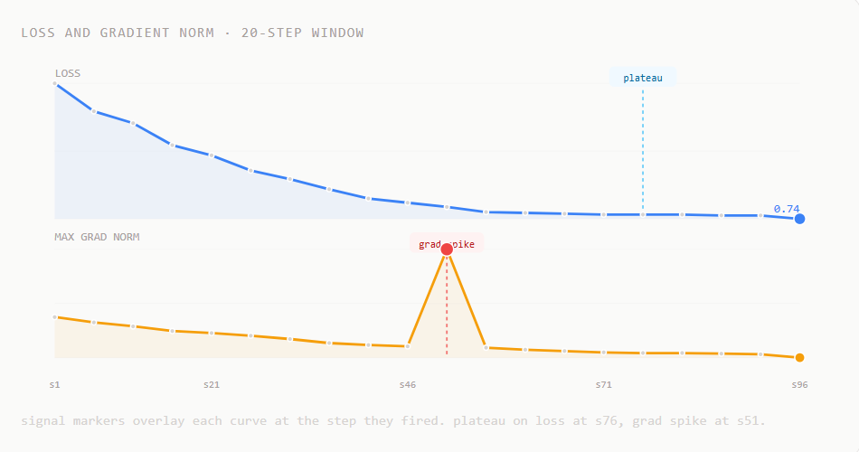
The training inspect system surfaces it in real time. A step event stream, loss, learning rate, gradient norms, per-layer breakdown, dead layer list, epoch index, feeds a signal engine that runs on each step as it arrives. When the engine detects a gradient spike, a loss plateau, a collapsed attention head, or the onset of loss divergence, a signal fires immediately with the specific metric and the exact step.

When training completes, the dashboard computes a model diff and a per-layer SAE feature diff, showing not just how loss moved, but which behaviors changed and which internal representations were rewritten.

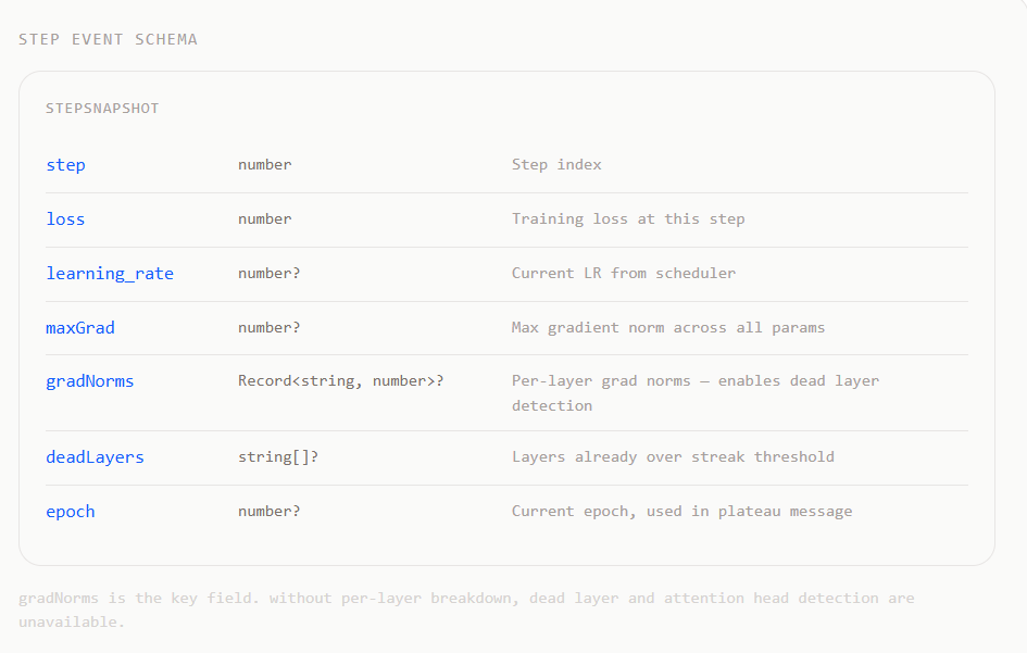
The system is agnostic to training framework. It consumes a flat step event schema: step index, loss, learning rate, max gradient norm, per-layer grad norms as a record, dead layer list, epoch index. No nested objects, no optional deep structures.

The per-layer grad norm breakdown is what enables the dead layer and attention collapse detectors. Without it, the engine observes only aggregate gradient behavior. With it, it names the specific layer that has collapsed and tracks how long it has been dead. The layer naming convention follows whatever key names the training framework uses; the engine applies a regex for attention layers and treats everything else as non-attention.

The signal engine is a pure function that runs on each new step snapshot. It takes the full step history plus two persistent streak maps, one for non-attention layers, one for attention layers and returns a signal if one fired, or null. The streak maps are the only stateful part: they persist across steps so that dead layer detection can track how many consecutive steps a layer has had near-zero gradient.

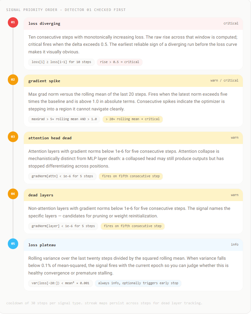
loss divergence and gradient spikes are checked first because they indicate active instability that may warrant stopping the run. dead layer and attention collapse are checked next, naming the specific failed components. loss plateau is last, it frequently describes healthy convergence rather than a problem, and its priority reflects that.

A 30-step cooldown prevents the same signal type from re-emitting continuously. A plateau that persists does not flood the feed. A gradient spike that resolves and re-occurs fires again after 30 steps, the second occurrence is a distinct event with its own context.

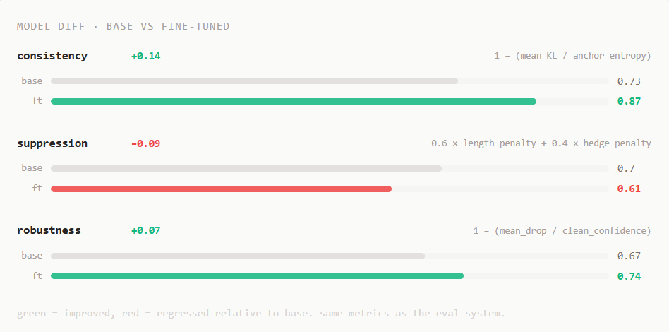
Three behavioral scores describe how the fine-tune changed the model from the outside: consistency score, suppression score, and robustness score. These are the same metrics from the eval system, applied to the base-vs-fine-tuned comparison. The base model is the reference; the fine-tuned checkpoint is the subject. The difference is the behavioral delta the training objective produced.

The robustness score is the most informative signal for factual fine-tuning. A fine-tune intended to reinforce factual knowledge should produce higher robustness on those facts, more confidence under surface corruptions of the relevant prompts. A robustness drop on target facts after factual fine-tuning means the model learned a surface pattern rather than a grounded representation.

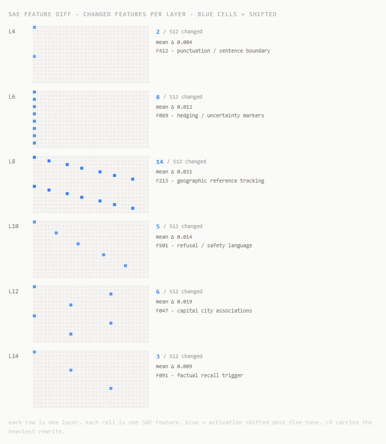
Behavioral scores describe the model from the outside. The SAE feature diff describes what changed internally. For each layer, the diff reports: how many features shifted activation between base and fine-tuned, the mean absolute activation delta, and the single feature with the highest delta.

Layer-level change density is the most informative aggregate. A fine-tune that changes 14 of 512 features at L8 and 2 of 512 at L4 is making a focused, deep rewrite not spreading surface changes across the network. The top feature per layer is where mechanistic investigation should start. If L10’s top shifted feature is F501 (refusal / safety language) and the training data had no refusal content, that warrants investigation in the model inspector.

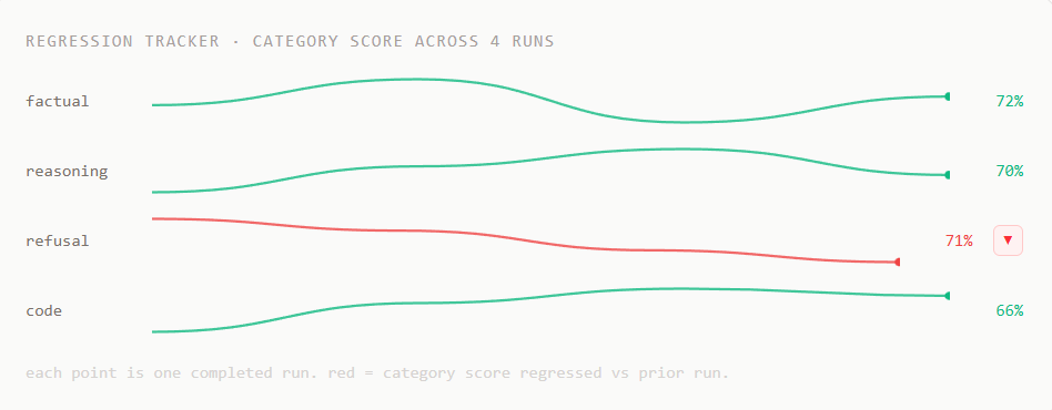
A single model diff shows how one fine-tune changed behavior relative to base. The regression tracker extends this across runs: every time a model diff arrives, category scores are appended to a per-category history so behavior can be tracked across all completed runs in the session.

A category that regresses more than five percentage points on the latest run is flagged. Detection is relative to the immediately prior run, not to the base, a score can look healthy against the base model while trending negatively across iterations. The tracker catches that drift where the raw diff cannot.

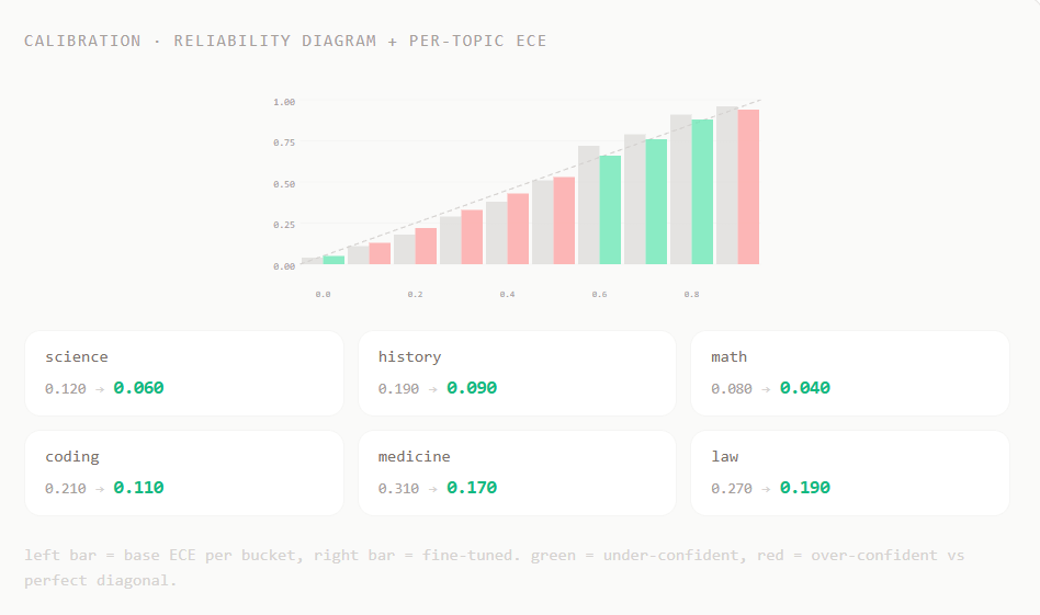
A model’s stated confidence and its actual accuracy can diverge in ways invisible from loss alone. A fine-tune can lower loss while making the model systematically overconfident. ECE measures that gap directly: it bins outputs by stated confidence, computes accuracy within each bin, and reports the mean gap between the two.

The calibration panel runs this comparison between base and fine-tuned using the training dataset as the evaluation set. The reliability diagram shows both models’ accuracy-per-confidence-bin as bar pairs against a perfect-calibration diagonal. The per-topic ECE table breaks the aggregate down by category, models trained on domain-specific data frequently improve ECE on the target domain while degrading it on adjacent topics that share surface patterns with the training examples.

The low-confidence row list surfaces inputs where the fine-tuned model assigns probability below a configured threshold. These rows are exportable directly as a labeled dataset for the next training iteration, the model’s own uncertainty becomes the selection criterion for the data that trains the next version.

Each finding from the training run is an entry point into a deeper investigation, not a terminal result. A dead layer signal at L6 step 61 is most usefully followed up by opening the fine-tuned checkpoint in the Model Inspector, going directly to L6 and running the causal trace to confirm whether that layer still contributes to outputs.

A suppression score that rises from base to fine-tuned opens a data investigation: the training dataset can be opened in the Data Inspector and the toxicity and PII modules run against the columns most likely to produce hedging signal.

The SAE feature diff provides the entry point for mechanistic investigation. Once the features that shifted most are identified and at which layers, the Model Inspector can be navigated directly to those features, their benchmark scores checked, the logit lens run, and steering applied to confirm their role. The diff turns post-training inspection from an open-ended search into a targeted inquiry.

The calibration panel adds a third path out of the training run, low-confidence rows exported as a labeled dataset for the next iteration. The regression tracker closes the loop in the other direction, confirming the next iteration did not trade one weakness for another. Together they make the training session the input to the next investigation rather than the end of one.