0029-5515/64/4/046014

Abstract

Typically the rampdown phase of a shot consists of a decrease in current and injected power and optionally a change in shape, but there is considerable flexibility in the rate, sequencing, and duration of these changes. On the next generation of tokamaks it is essential that this is done safely as the device could be damaged by the stored thermal and electromagnetic energy present in the plasma. This works presents a procedure for automatically choosing experimental rampdown designs to rapidly converge to an effective rampdown trajectory. This procedure uses probabilistic machine learning methods paired with acquisition functions taken from Bayesian optimization. In a set of 2022 experiments at DIII-D, the rampdown designs produced by our method maintained plasma control down to substantially lower current and energy levels than are typically observed. The actions predicted by the model significantly improved as the model was able to explore over the course of the experimental campaign.

Export citation and abstractBibTeX RIS

The termination phase of a shot is an essential part of tokamak operations for all machines present and future. In this phase, the plasma current is decreased as much as possible while attempting to avoid disruptions until confinement is eventually lost. Currently, a large fraction of the disruptions that occur during machine operations occur during this termination phase. For the current generation of machines, disruptions are usually tolerable because they cause little damage. For ITER and future fusion reactors geared toward power generation, disruptions pose a significant concern. At ITER, the specified total number of major disruptions assumed for the design of ITER components is 3000 (equating to 10% of the anticipated full-performance pulses) [33]. Special emphasis is placed on avoiding vertical displacement events. In an analysis of future tokamak power plants [27], it was found that ‘the disruption handling requirements for achieving $\lt$ $100 MW h⁻¹ LCOE are extreme’. Therefore, identifying operating regimes and control strategies that reduce disruption risks is vital in order to remain within these limits. The physics of disruptions is poorly understood—most progress of physics during disruptions has been made by solving the extended magnetohydrodynamic (MHD) equations with codes like NIMROD [39] in order to explain observed phenomena. What is more, as outlined by [11, 22], disruption prediction is a harder task still due to the disparate disruption causes, so empirical models are the state of the art and are far from perfect [15].

In the termination (or rampdown) phase, a number of concurrent changes must be made to the plasma state: the plasma current must be decreased to zero, the auxiliary heating power must be removed (which will precipitate the H to L-mode back transition and a consequent decrease in kinetic energy if it has not already occurred), and density must decay. While these changes are occurring, a number of operating and stability limits of the plasma must be respected in order to avoid disruption and consequent damage to the device. Of paramount importance is the maintenance of vertical stability (VS), which is related to the inductance $\ell_i$ , $\beta_\mathrm{p}$ , and the elongation κ as discussed in [44]. The VS limit differs across machines, and at DIII-D benefits from the presence of poloidal field coils located close to the plasma that can respond quickly. The Greenwald density fraction $f_\mathrm{GW} = \frac{n \pi a^2}{I_\mathrm{p}}$ [17] is another key quantity of interest during the rampdown and can cause disruptions when it exceeds 1 as $I_\mathrm{p}$ decreases unless density concurrently decreases. The Greenwald limit is an idealized quantity and work such as [16] continues to sharpen our understanding of density limits on different devices under various conditions. Another potential concern during rampdown is the presence of a variety of MHD instabilities in the plasma, which can cause the plasma to disrupt if they grow too large. Finally, there is a possibility that the plasma undergoes a radiative collapse, where there is no longer sufficient kinetic energy to maintain stability. One possible cause of this is excessive radiation due to impurity accumulation. In this work we explore the optimization of rampdowns using a Bayesian optimization (BO) strategy. Before further explaining the contributions of this paper, we first give some background on BO in the context of machine learning (ML).

1.1. Related work

1.1.1. Rampdown optimization.

Prior works [41, 44] have addressed the termination phase through optimization and study via models derived from first principles. In this work, we aim in contrast to address this problem through an ML based method for rampdown trajectory design. In [44], a large scale analysis of the components of stability of rampdowns was conducted across many of the world’s tokamaks; here, the goal was to describe and analyze the key physical phenomena that determine whether a rampdown is successful or disrupts prematurely. The authors identify the relationships between the change in elongation, decrease in power, and decrease in current that underlie the control developments in this work. Another study was conducted in [41], where numerical optimization was conducted over rampdown trajectories using the RAPTOR simulator. The plasma was successfully ramped down using the design given from the optimization solution on both the TCV and ASDEX Upgrade tokamaks. The key differences between that work and this one are that here there is a data-based approach to rampdown design rather than a simulation-based and there was a large-scale experimental campaign at DIII-D in contrast to study of a pair of shots on different machines. In [3], the authors develop an emergency shut-down procedure which involved transitioning to a limited topology in order to maintain control down to a safe current level. Our work addresses the nominal rampdown in a similar spirit, but we use an ML based methodology to design the trajectory. Finally, in [15], the authors propose an ML-based controller which predicts disruptivity. During the rampdown phase, future disruptivity is predicted in real time. If at any point the disruptivity prediction exceeds a threshold, an off-normal response is triggered that begins a fast rampdown of the plasma current in order to disrupt at a safer level. This feedback control mechanism is complementary to this work—we focus on the design of feedforward trajectories which avoid disruptions in advance while this method reacts in a closed-loop fashion.

1.1.2. BO.

1.1.3. Learning-based control in fusion.

Typically in learning-based control, an agent interacts with an environment by alternately executing actions and receiving observations. The agent then adjusts its decision-making policy based on the information it has collected in a way which aims to optimize some objective. In this work we use ‘agent’ to refer to a generic decision making entity (as in [25]) though it is most often used to refer to the reinforcement learning setting. In the broader ML world, the greatest successes of learning-based control methods have inevitably come when the agent has the ability to collect a large number of samples using its current policy in the ground-truth environment. This has happened most notably in games like Atari [28], Go [36], and Chess [37] but also plays out in domains where there is a fast and accurate simulator of the system. In [12], reinforcement learning was applied to a simulator of current and shape dynamics in order to find a policy which was successfully able to achieve a desired shape on the TCV tokamak. However, shape control is typically achieved using hand-designed and more interpretable controllers [45] for the same reason that the simulation was accurate: the underlying dynamics of shape control are relatively easy to model. For kinetic control or other more challenging problems, the direct sim-to-real transfer approach may be more difficult. To address this, works like [7, 35] learn a policy from dynamics models trained on previously logged data collected by the experiments that have been run on KSTAR and DIII-D, respectively. These works fall under the so-called ‘offline reinforcement learning’ setting [24]; there are inherent challenges associated with this setting such as the fact that the training data was generated by some other policy (fusion scientists running experiments) rather than the agent. Another direction that has been explored is that of finite-set control with a learned model as in [1], where the controller predicted future states for a finite set of actuator settings and chose the one which was predicted to be closest to the target temperature profile. Yet another learning-based control method was deployed in [15], where a decrease in injected power was precipitated by a learned disruptivity model. In each of these works, a model was fit to a static dataset and used to make control decisions for the tokamak. As tokamak time is exceedingly limited, it is often infeasible to train controllers in an online fashion (on the machine, with opportunity for the agent to learn from its previous experiences) for fusion applications.

1.2. Contributions

In this work, we took advantage of a rare exception to the preceding statement: during the 2022 operations on the DIII-D tokamak we undertook a (relatively) large-scale study of online data-driven rampdown designs. This was made possible by our ‘piggyback’ experimental design in which we were able to vary the parameters of rampdowns at the end of shots for which the primary experimental data was to be collected during the flat-top phase. After choosing a parameterization for a feedforward control trajectory and a cost function for the desired rampdown behavior, we projected historical DIII-D data onto our action space and trained probabilistic models that predicted the cost incurred by the rampdown from the action chosen. We first executed the optimal action according to the model several times. Then, we began choosing actions according to a handful of data acquisition functions taken from the BO literature in order to efficiently explore the design space of rampdowns. After running a few dozen trials in this way, we executed the optimal action according to an updated model several times.

With the caveat that we could not control the initial conditions of the rampdowns in our tests, we found that when compared against the other shots at DIII-D (either those from the same experiments or the broader dataset) our rampdowns were significantly better at reaching low currents prior to disruption with a mean current at disruption 2.5× lower than the DIII-D average. The rampdown designs improved over the course of our experimentation as a general trend and that the final optimum outperformed the initial optimum found, showing that the exploration was helpful in improving our estimate of the optimal rampdown. Our methodology is fairly general and could in principle be used for other feedforward trajectory design problems in plasma control in the future.

In section 2, we present the rampdown optimization problem setting and discuss the assumptions made in order to simplify our procedure. Section 3 describes the methods used, including data processing, ML methods, and our experimental protocol. Section 4 presents the results of our initial modeling exercise as well as a quantitative discussion of our experimental results. In section 5, we analyze pairs of shots from the test and control set in order to understand what might be driving the observed differences in performance. In acknowledgments section, we conclude by discussing the work in a broader context and give an idea of future directions.

At a high level, our approach is simple: given an action space $\mathcal{A}$ and a cost function C we aim to find the action $a = \operatorname{arg min}_{a \in \mathcal{A}} C(a)$ by making queries to C using various actions a. In order to do so, we need to find actions which efficiently search the space of possibilities and take into account the values of C obtained by executing various actions. At the ith trial, the action a_i is chosen by approximately maximizing some criterion $\alpha_i(a)$ which we refer to as an acquisition function that can be derived from a probabilistic estimate $\hat{C}_i$ of the cost function C. We execute a_i for one or more experiments. Then the we run a script to ingest the additional data from the tokamak, process it so that it can be use to fit another ML model $\hat{C}_{i + 1}$ , and generate a new action by optimizing the acquisition function $\alpha_{i + 1}$ . By iterating this process for n iterations we aim to discover an action $\hat{a}^* = \operatorname{arg min}_{a\in \mathcal{A}} \hat{C}_n(a)$ that is the ‘best guess’ for the best action design. Though this work focuses on the application of this general loop to the rampdown design problem, it is in principle applicable to a much wider set of problems. There is a diagram of the overall loop in figure 1.

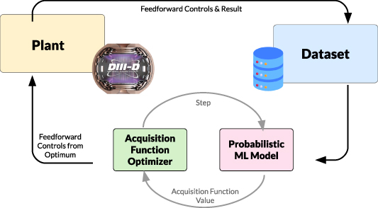
Figure 1. Refer to the following caption and surrounding text. — **Figure 1.** Diagram of overall method. Here, the process of executing the actions that optimize the acquisition function and observing their results is shown.
Download figure:
Standard image High-resolution image

First in section 2.1, we describe the choices for $\mathcal{A}$ and C. Next, in section 2.2, we describe how we acquire and process the data in order to input it into the ML model. Then, in section 2.3 we discuss the ML methods used to estimate C and the acquisition functions used in the paper. Finally, in section 2.4, we describe the protocol for executing actions on the DIII-D tokamak in a series of piggyback experiments spanning most of 2022.

2.1. Problem setting

We address the rampdown problem as a BO problem where the action space $\mathcal{A}$ is the space of designs for rampdowns and the cost function aims to capture the damage that might be done by a particular rampdown. In making this choice, we explicitly ignore the problem of context—that is, we mostly ignore the state of the plasma at the time the rampdown is initiated and search for a specific rampdown design rather than a function mapping the plasma state to a rampdown design. This choice was made for simplicity of modeling and optimization, but we also note that it is not generally possible to know exactly the state of the plasma at the end of the flat-top phase prior to the shot. It also was made in light of the fact that we would be running these experiments in a piggyback capacity after other experiments at DIII-D and therefore we would have very little control or even information about what the state of the plasma would be at the end of the flat-top phase. We also are only addressing feedforward control and explicitly leaving the feedback control to existing systems. This choice allows the flexibility to explicitly change the controller behavior based on new information without recompiling the plasma control system. We give a diagram of the overall loop in figure 1.

In order to specify the optimization problem, we must define an action space and an objective function.

2.1.1. Action space.

Stemming from prior work [3], we decided that it was most practical to vary three actuators:

power injected from the neutral beams (pinj)
current (Ip)
elongation of the plasma shape (κ).

As a rampdown design requires all of these to be varied in time, we needed a way to parameterize the trajectory of each of these actuators over time starting from the programmed beginning of the rampdown. As we aimed to conduct piggyback experiments, we explicitly do not consider any changes to shot programming prior to the beginning of the rampdown phase. After considering a handful of methods, we decided on a piecewise linear (PWL) function for each, which we represented with three parameters: delay (t₀), rate (r), and duration (Δt), which we collectively call θ. We depict these in figure 2. This parameterization also leaves as a free variable the initial value x₀ of each trajectory as these may vary depending on the design of the shot at rampdown. When we execute a PWL action parameterized by θ in a piggyback, we use the value of x₀ from the beginning of the rampdown in the nominal shot trajectory in order to concretely generate the feedforward rampdown trajectory. Then for a particular signal $x_\theta(t)$ starting at time t = 0 with initial value x₀, delay t₀, rate r and duration Δt the value is given by

Equation (1)

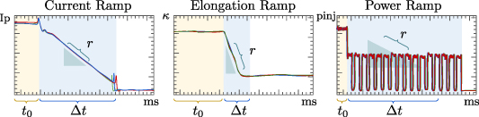
Since we need a PWL representation of the action for each of our three actuators, our action representation $a\in \mathcal{A}$ has a total of nine parameters $a = [{\theta_{\textrm{pinj}}}, {\theta_{\textrm{Ip}}}, {\theta_{\kappa}}]$ that represents the 3D time series $[x_{\theta_{\textrm{pinj}}}, x_{\theta_{\textrm{Ip}}}, x_{\theta_{\kappa}}]$ .

Figure 2. Refer to the following caption and surrounding text. — **Figure 2.** Depiction of an example action in our piecewise linear parameterization for current, elongation and injected power. This example is a stylized drawing of shot 188823.
Download figure:
Standard image High-resolution image

2.1.2. Objective function.

The primary goal of a rampdown design is that it is safe against disruptions. In particular, disruptions at high levels of current are of concern to operations at tokamaks as well as the uncontrolled release of the various forms of electromagnetic and thermal energy stored in the plasma. In all applications of ML, the design of the objective is especially critical. One of the fundamental choices is whether to shape the objective function in order to encourage behavior that is thought to lead to outcomes consistent with the ultimate goal. In other words, one might add an instrumental goal to the objective function in the hopes of encouraging behavior that leads to the ultimate goal. This is often done in artificial intelligence (AI) research contexts [19] by e.g. adding a reward for advancing toward a target state even though the objective is actually only to attain it. In this work, we used an objective function with some reward shaping with the ultimate goal of reducing the current at disruption time. Our cost function for an action a as described above is

Equation (2)

where ${t_\mathrm{D}}$ is the time of disruption (as marked by the time at which the current quench occurs), $x_{\theta_{\textrm{Ip}}}({t_\mathrm{D}})$ is the plasma current at the time of disruption, $a_{\textrm{minor}}^{t_\mathrm{D}}$ is the minor radius at the time of disruption, B is the magnetic field, $W_{\textrm{MHD}}^{t_\mathrm{D}}$ is the MHD energy of the plasma at the time of disruption, $q_{95}^0$ is the safety factor 95% of the way to the edge at the beginning of rampdown, and $q_{95}^t$ is the same safety factor at times during the rampdown.

The first two terms of the objective are the electrical and MHD energies of the plasma. These relate to the objective of controlling the plasma to as low of an energy content as possible before a disruption. The third term penalizes any rampdown where the safety factor, q₉₅, drops below its initial value over the course of the rampdown. This term is an example of the reward shaping mentioned earlier: as q₉₅ is a key determinant of the stability of the plasma [8], we encourage our agent to keep it from decreasing. Additionally, this reward is roughly unit-scale, which simplifies the modeling process.

2.2. Offline then online data processing

In order to achieve an initial offline estimate of the objective function C, we fit a model to historical data from DIII-D. The data processing consisted of three steps: collection, preprocessing, and featurization. In the collection phase, we pulled data about historical DIII-D shots numbered 120000–188814, which run from 2004 to April 2022. from the MDSPlus database as in [1] in 50 ms windows. In particular, we collected the information about the action space: target plasma current, injected power from the neutral beams, and elongation as well as for the cost function: safety factor near the edge (q₉₅), minor radius, and MHD energy as computed by EFIT01. For the cost function we also collected the time of disruption (as marked by the current quench) and the plasma current at that time. In order to do so, we used a technique developed in [3]. The time of current quench is determined by searching for dIp/dt passing a very high threshold (−14 MA s⁻¹) for reduction in plasma current after which the plasma current never recovers. The beginning of this very fast final Ip drop is the time which the current quench begins, and is used for the current quench time in this work. Our method then double checks that this drop was not programmed as part of the desired trajectory of the shot. In some cases the plasma recovers after a very large transient event. The code ignores this phenomenon and skips forward to the final (actual) disrupting event.

Finally, we also collected the times at which the rampdowns were programmed to start in order to know at what time the agent could have begun to modify the controls.

In order to make sure that the data were usable for ML, it was preprocessed into a form that made it suitable for featurization. Much of this involved removing shots which were unsuitable for use in this study. We removed shots for which any of the following occurred:

Shot disrupted prior to originally scheduled rampdown or within 50 ms of rampdown beginning.
Shot data in relevant fields contained at least four consecutive NaNs (lasting 200 ms).
PWL action projection could not achieve sufficient accuracy (see below).

This left us with 1173 shots in the original offline dataset from which to perform regression. This data cleaning procedure was conservative and led to shots being excluded which otherwise could have been used. This is important in the experimental section where certain experimental shots did not pass data filtering checks and are therefore excluded as in figure 5. As the experiments progressed all subsequent shots were appended to the dataset including but not limited to those where the rampdown was designed by the model.

2.2.1. Projecting historical data to the PWL action space.

For each shot retrieved from the DIII-D database, actuator data is represented as a time series $\{u_i\}_{i = 0}^k$ with u_t the scalar values of the actuator every 50 ms. For shots which disrupted during the rampdown the lengths for the action representation were padded as if they had gone to their intended conclusion and disrupted at 50 kA. In order to use PWL representation for the action space, it was necessary to find some PWL parameters that approximately corresponded to the time series retrieved for each actuator in each shot. Thus we solved the following optimization problem with the curve fitting library taken from scipy [43], which uses the trust region reflective algorithm [5]:

Equation or symbol description not available

This optimization problem is a projection of the time series of each actuator onto the space of PWL functions. As these coefficients found were to be used as features for the subsequent ML estimation, we discarded the shots for which the projection induced substantial error. Concretely, these were shots for which $\frac{||x_{\theta}(t) - u_t||_2^2}{||u_t||_2^2} \gt 0.1$ . This was the case for at least one signal in 34% of the data. The dataset $D_n = \{(a_i, c_i)\}_{i\in[n]}$ consisted of the observed actions after all preprocessing as well as the computed costs.

After performing this optimization and filtering, we fit an ML model for C and choose an action as described below.

2.3. ML methods

As discussed in section 1.1, there has been a huge amount of work done in the ML community addressing the BO setting. The standard approaches involve uncertainty-aware regression to learn the function C from observations $(a, C(a))$ . The specific types of uncertainty required are determined by the acquisition function $\alpha_i(a)$ being used.

2.3.1. Uncertainty-aware regression techniques.

There is a substantial literature of uncertainty-aware regression techniques [2, 30]. This work relied on three representations of predictive uncertainty: epistemic uncertainty, aleatoric uncertainty, and posterior sampling. Epistemic uncertainty is the uncertainty in predictions that can be reduced by making observations and performing inference. Aleatoric uncertainty is the irreducible uncertainty in a prediction, often because the system is itself stochastic. Due to the many unobserved features of the tokamak at rampdown time, there is substantial uncertainty that could be reduced given perfect observations but is not captured in the data presented to our model. For modeling purposes, this is treated this as irreducible given our assumptions. Posterior sampling is a bit different—given some approximate prior belief over cost functions P(C), and a set of observations D_n , we can update our beliefs to an approximate posterior $P(C \mid D_n)$ and sample from it. This process can be interpreted as choosing from the set of functions that are consistent with the observations D_n given prior knowledge. Many of the tools developed in BO deal with settings where the black-box function can be fit well by a Gaussian process regression with some kernel. Even when using empirical techniques like maximum marginal likelihood kernel fitting, we were unable to find a kernel that gave reasonable predictive accuracy on our data.

Instead, we used both multilayer perceptrons (MLPs) (following [29]) implemented in JAX [4] and gradient boosted trees (GBTs) taken from the Catboost package [13] alongside probabilistic variations and ensembles composed of these units. In their standard forms, neither MLPs nor GBTs estimate uncertainty. However, this can be easily solved for each by having the model output the mean (which we write $\hat{C}(a)$ ) and standard deviation $\hat{\sigma}(a)$ of the response variable and training them via maximum likelihood [26]. We follow [10] in using $\hat{\sigma}(a)$ for an estimate of the aleatoric uncertainty $\sigma_\mathrm{a}(a)$ , while the standard deviation of the mean predictions of ensemble members $\hat{C}_i(a)$ can be interpreted as an estimate of the epistemic uncertainty $\sigma_\mathrm{e}(a)$ . One also can sample a single ensemble member $\hat{C}_i(a)$ as an estimate of a function sampled from the posterior. At every iteration, the model was trained using all observations that were part of the dataset. Ensembles consisted of ten members trained on bootstrapped data sampled with replacement from the training set.

To address the lack of a clear hypothesis over the objective function C, we employed a rotational strategy with different function approximators for each acquisition function. As discussed below, this involved periodically switching between various approximators to align with the requirements of each acquisition function. Concretely, we alternated between MLPs and GBTs and then choose the probabilistic and/or ensemble variant that would provide the uncertainty estimate required by the acquisition function being used (see table 1 for these).

Table 1. Data acquisition functions and the corresponding uncertainty estimates required.

Acquisition function	Uncertainty estimate required	Functional form of α
Optimum	None	$-\hat{C}(a)$
Thompson sampling	Posterior sampling	$-f(a), f \sim P(C\mid D)$
LCB	Epistemic uncertainty	$-\hat{C}(a) + \beta \sigma_\mathrm{e}(a)$
UCB-LCB	Epistemic & Aleatoric uncertainty	$-\hat{C}(a) + \beta_1 \sigma_\mathrm{e}(a) - \beta_2\sigma_\mathrm{a}(a)$

2.3.2. Acquisition functions.

In order to acquire data that will facilitate black-box optimization, we use the probabilistic estimates of the cost function discussed in the previous section to compute various acquisition functions α_i and collect observations located at the optimum of these functions. Besides choosing the optimum of the estimated cost function itself, we used Thompson sampling [32], lower confidence bounds [40], and upper/lower confidence bounds as acquisition functions. Thompson sampling relies on the fact that choosing the optimum of a function sampled from the posterior is equivalent from sampling from the posterior over optima. Lower confidence bounds use an optimistic decision rule to choose points at which the model is either overconfident or correct in its optimism, thereby ruling out parts of the design space which could potentially be good. Upper/lower confidence bounds additionally include a penalty for areas of the design space that are estimated to be highly noisy. As shown in table 1, each of these acquisition functions requires a particular type of uncertainty estimate.

Each of these acquisition functions has shown state-of-the-art performance on some BO problems. Given the uncertainty about which function would best suit this application, we adopted a strategy inspired by [18]: cycling through these functions for each subsequent trial. This approach involves selecting a model which provides the appropriate uncertainty estimate for the specific acquisition function in use at any given trial.

2.4. Piggyback experiments

Throughout the course of 2022, we conducted a campaign of piggyback experiments executing various rampdown designs after the conclusion of the flat top phase. For experiments for which the session leader (SL) was amenable to our work, the mainline experiment could tolerate some disruptions, and the authors were available, we collected data based on executing actions chosen according to an acquisition criterion with maximally up-to-date data. We also made sure to collect data which used the default rampdown in order to be able to see a useful control set. At DIII-D the nominal rampdown evolves over time as SLs modify it, but the default strategy has been a decrease in current at 1 MA s⁻¹ and a complete shutdown of beam power very close to the start of rampdown. The shape is changed to a low-elongation and limited plasma shape around 100 ms into the rampdown. There are often small changes in the vicinity of this design. Within an experiment, we would first allow the SL to run with no modifications on our end until they were able to achieve a plasma that lasted until the programmed time of rampdown. For several experiments, this proved difficult and we were unable to run. Once several trials successfully reached the rampdown phase we programmed in an action generated by optimizing an acquisition function and executed it several times. Once it had executed several times, we ran our scripts for ingesting and preprocessing additional data, generated another action, and executed it as well. This process proceeded across several run days in 2022.

3.1. Initial modeling results

The first step was to fit an estimate of our cost function $\hat{C}$ to the offline dataset D. We initially considered models ranging among linear regression, k nearest neighbors, Gaussian processes, GBTs, and traditional MLPs. Hyperparameter tuning and model selection was conducted using five-fold cross validation on a training set consisting of 80% of the training data. GBTs and MLPs performed best on cross validation. The MLP with learning rate of $3\times 10^{-4}$ worked well as did CatBoost [13] with out-of-the-box settings. GBTs achieved 74% explained variance on the test set and the MLPs were slightly worse at 72%. As can be seen in figure 3, the optimum found in the initial model calls for a moderately aggressive current rampdown (close to 1.8 MA s⁻¹) along with modest change in elongation and an aggressive decrease in beam power (80 MW s⁻¹, an immediate shutdown). The optimum is not as low-cost as the lowest-cost elements due to the fact that the model does not predict extreme values as well. An analysis of the feature importances showed that the ramp rate and duration for current were the most important features used to explain the cost function, a result in line with expectations.

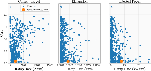
Figure 3. Refer to the following caption and surrounding text. — **Figure 3.** Optimization of a learned model using offline data only. This figure depicts a GBT model mapping θ to the cost function to all high-quality examples available prior to our experimental campaign and optimized it via grid search over θ. The plots show the historical observations and the optimum found for three components of θ.
Download figure:
Standard image High-resolution image

3.2. Real-world performance of online BO

After our offline modeling we ran 41 piggyback shots with 16 different synthesized actions across eight different run days at DIII-D in 2022. The actions were synthesized by optimizing acquisition functions defined over the GBT and MLP models as described in section 2.3. We aimed to answer two questions: (1) did our model synthesize better rampdowns than the default at DIII-D? and (2) could our exploration strategies cause the rampdown designs to improve over time through our trials? In both cases, the answer was yes, with some complexity in the answer to (2).

To address the first question, we determined two potential control sets: all rampdowns on DIII-D after 2015 (wide control) and all rampdowns taken from the same miniproposal (a document which references a particular experimental allocation in the DIII-D procedures) as our test shots (same-MP control). After removing all shots with missing data, the wide control set was 11 047 shots, the same-MP control set was 25 shots and the test set was 29 shots. The latter two covered a wide range of plasma conditions, with flat top current ranging between 0.6 and 1.6 MA in the test set and 0.55 and 1.8 MA in the same-MP control set and β_N ranging between 0.6 and 2.4 in the test set and 0.4 and 2.2 in the control set. The observed currents at disruption as well as the computed costs for these three sets are shown in figure 4. It is clear by inspection that the shots in the same-MP control disrupted at a similar distribution of plasma currents to the broader baseline of DIII-D shots. However, in the test shots, our method was able to perform significantly better than was observed in either control set. The mean current at disruption in the test set, 134 kA, was 2.5× smaller than the mean current at disruption in the control set (336 kA) and 2.9× smaller than that of the same-MP control (389 kA).

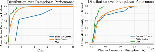
Figure 4. Refer to the following caption and surrounding text. — **Figure 4.** Performance of comparison sets of rampdowns on cost and current at disruption. These are empirical cumulative distribution functions, so e.g. the median of the observed samples will be the value on the horizontal axis where the curve crosses 0.5 on the vertical axis.
Download figure:
Standard image High-resolution image

After the conclusion of our experimental campaign, we performed statistical tests to assess the possibility that our results were the result of random chance. Ideally, we would have chosen a significance threshold for our statistical results prior to beginning our experimental campaign. However, we did not do so and can only comment on results after the fact. Based on the p-values observed in table 2, which give the probability that differences of at least this magnitude could be observed between samples generated from the same process, it is highly unlikely that our results were generated by random variation. We also compute the modified Cohen’s d, a measure of the effect size taken by normalizing the difference between means of two samples by the standard deviations. Typically, 2 denotes a large effect size [34] and each of our comparisons attains that threshold.

Table 2. Statistical tests of rampdown performance. We used the Mann–Whitney U-test on the disruption currents and costs observed in our experiments to compute the p values shown here. We report the modified Cohen’s d for effect sizes.

p-value/effect size	Same-MP control	Wide control
Current at disruption	0.027/−2.77	$1.7 \times 10^{-6}$ /−10.97
Cost	$9.9\times 10^{-5}$ /−2.72	0.018/−2.79

In particular, it was more clear for the same-MP control that the cost attained by our method was an improvement compared to the current, while the reverse was true for the wide control. This might have been due to the fact that the same-MP control contained more recent shots where the rampdown has been optimized more for current but not the cost function, leading to improved performance on the former metric but not the latter relative to the wider control set. It is again important to note that these results come with the caveat that we could not control much of the experimental process due to the piggyback experiment design.

Figure 5 shows the performance of the test actions over time. The results are mixed. There is no clear trend in the series of costs (blue) and in fact the last datapoints that are not missing from our time series have fairly high costs compared to the others (some investigation showed us that this was due to a drop in q₉₅ immediately at the beginning of the rampdowns). However, the currents at disruption at the end of each rampdown (red) show a clear downward trend as the experiments proceeded. This trend suggests that over time the model learned actions that were more reliably able to bring the shot down to a very low current prior to disruption. One important caveat to note is that these are modest sample sizes and we do not have perfectly controlled conditions so it is possible that our results were the result of statistical fluctuations or unobserved factors.

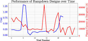
Figure 5. Refer to the following caption and surrounding text. — **Figure 5.** Costs and disruption current observed in test group experiments as trials were conducted.
Download figure:
Standard image High-resolution image

The previous section gave quantitative results of the rampdown experiments. This section presents qualitative results and gesture at how the model may have modified the rampdowns in order to avoid disrupting at high current.

4.1. Analysis of selected shots

Figure 6 shows three examples of shots from the test and same-MP control sets in our study that were taken from the same experiment. The left example depicts a pair of shots (a control shot, 192252, and a test shot, 192244) where the control shot disrupted at around 700 kA. Though they started from similar initial conditions, the test shot had a slightly higher ramp rate on Ip and power than the control shot. The control shot experienced a n = 2 mode that locks around 5200 ms and led to an early disruption. The test shot was able to last longer without such issues until the decreased current caused the Greenwald fraction to increase and cause a disruption at a much safer current level. Notably, the test shot 192244 is the shot with the highest current at disruption in our test set and thus gives a mild failure case of our method.

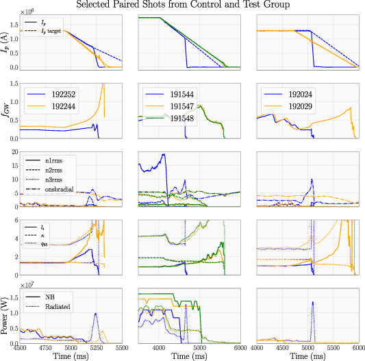
Figure 6. Refer to the following caption and surrounding text. — **Figure 6.** Selected paired shots from the test and control sets. Orange is test group and blue/green are control. Shot numbers are given in the second row.
Download figure:
Standard image High-resolution image

The second example shows three shots: the control shot 191544 and the test shots 191547 and 191548. It seems likely that 191544 disrupted due to an already-existing n = 1 mode that was not present in either test shot 191547 or 191548. This example highlights the difficulties in this piggyback experimental setup: as we were not controlling the conditions of the flat top we cannot reproduce the conditions at the beginning of rampdown and reproduce the challenges encountered. Though these two examples here of very similar rampdowns with slightly slower ramps show good results it is impossible to know whether they would have survived if given the initial conditions of 191544.

The final example shows a combination of exogenous and endogenous factors causing the plasma to safely ramp down. The control shot (192024) disrupts almost immediately upon beginning the rampdown due to what appears to be a locked n = 1 mode. The time of the rampdown was slightly moved up by the flat-top operators, and our method output a more gradual IP ramp rate. Together these changes were sufficient to cause the shot to ramp down smoothly to minimal plasma current.

4.2. Action selection across experimental campaign

We also inspected the actions output by the acquisition function optimization in order to understand whether there were any patterns observable from the data. Figure 7 shows some components of the action space of particular interest: the rates of change suggested by the model for power, current, and elongation. From this, it is clear that the model quickly gives up on varying the elongation of the model. This could be because DIII-D has vertical control coils that are very capable and close to the plasma and therefore the model does not find a decrease in elongation necessary to maintain VS. A similar study on a different device with less VS control (ITER, for example) might therefore lead to a rampdown design that relies more heavily on elongation than ours. In many shots, there is an unactuated decrease in elongation as current drops (see figure 6 for examples) and perhaps the model was able to infer the necessary relationships between the control requests and the eventual outcomes. The model explores a range of aggressive $I_\mathrm{p}$ ramp rates prior to converging to a healthy but less aggressive ramp rate around 1.2 MA s⁻¹. The model also widely explores various settings for the rate of change of power. The model seems to be somewhat confounded by the range of initial power settings at the start of rampdowns, which are part of the context for each shot that the model does not recieve. If the context had been included in the model, we would expect to see a more convergent process for injected power. This is a three-dimensional slice of a nine-dimensional action space so there are six additional axes of exploration not shown here. In the future we hope to extend these methods to include context and in fact to potentially move to closed-loop control in order to respond to developments in real time. We will also potentially attempt to control density in order to address an unaddressed cause of disruptions (the Greenwald limit) from the current setup.

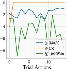
Figure 7. Refer to the following caption and surrounding text. — **Figure 7.** Rates of change chosen by models over time for current, elongation, and NBI power.
Download figure:
Standard image High-resolution image

We conclude with a discussion of piggyback experiments using ML more generally. As ML methods are data-hungry and tokamak time is scarce, it is necessary to either use offline data or to find applications like this one where nonstandard opportunities are available to run experiments. We aimed to keep the experimental and ML protocol as constant as possible as experiments progressed. As discussed in section 3, reward shaping actually made experiments and analysis more difficult to run. We encourage practitioners trying similar setups in the future to keep things as simple as possible in all aspects, including the data used in decision making and reward computation, the codebase for ingesting data and updating the models, and in the success criteria. It was crucial to keep a fixed experimental protocol on our end in the face of the variation inherent in tokamak operations. ML-driven control of tokamaks is a promising direction and we hope that our study design is instructive alongside our results. In settings where protocols for rampdowns are not available, as with new machines that do not have these procedures, these methods might prove particularly valuable in exploring possible trajectory designs.

In the previous section, we discussed the ‘convergence’ of certain components of the actions chosen to some reference values. There is a large literature [9, 14, 32, 40] discussing the rates of convergence of the various data acquisition methods used here in formal settings. Many of them can be tuned in order to achieve a desired confidence bound or even to work backward from a known horizon of experimentation. Throughout our study, we were highly uncertain about the number of trials we would be able to execute due to scheduling and machine operation questions that are familiar to all tokamak experimentalists. This made the question of how to tune our acquisition strategy slightly more difficult.

This work aimed to find a rampdown trajectory that improved the existing one at DIII-D by trial and error using strategies from black-box optimization. In experiments over the course of 2022 we conducted trial rampdowns as piggybacks and updated our model with new observations as they came in. Our rampdowns were able to bring the plasma current down to an average value 2.5× smaller than is typical at DIII-D and, based on our statistical tests, our results are unlikely to be due to chance. However, as we could not control the plasma state at the beginning of rampdown it is difficult to decouple disruptions due to physical phenomena present at this time from disruptions due to poor control.

One exciting direction for future research is in attempting a similar experimental campaign without the benefit of the existing DIII-D database but perhaps with the use of first-principles driven simulators such as those being used for the development of ITER [23] and SPARC [31]. Although the specific rampdown design we developed in this work is unlikely to transfer to those devices, it is possible that a procedure like this one could be used to support the commissioning of rampdowns at each. The efficient and robust commissioning of rampdowns for these devices will be an important part of their successful operation within disruption constraints. Simulating those conditions could help us understand the effectiveness of these methods in a more realistic setting. With all this considered, we see ample opportunities for additional work of this nature, both in continuing to optimize and better understand rampdowns on DIII-D and at other machines and in applying active ML methods to other control tasks in fusion research.

We would like to acknowledge the generosity of the SLs who allowed us to piggyback on their experiments in order to collect the data for this work. Without their generosity, this work would not have been possible. This material is based upon work supported by the US Department of Energy, Office of Science, Office of Fusion Energy Sciences, using the DIII-D National Fusion Facility, a DOE Office of Science user facility, under Awards DE-AC02-09CH1146 and DE-FC02-04ER54698. This work was also supported by DE-SC0021414 and DE- SC0021275 (ML for Real-time Fusion Plasma Behavior Prediction and Manipulation).

This report was prepared as an account of work sponsored by an agency of the United States Government. Neither the United States Government nor any agency thereof, nor any of their employees, makes any warranty, express or implied, or assumes any legal liability or responsibility for the accuracy, completeness, or usefulness of any information, apparatus, product, or process disclosed, or represents that its use would not infringe privately owned rights. Reference herein to any specific commercial product, process, or service by trade name, trademark, manufacturer, or otherwise does not necessarily constitute or imply its endorsement, recommendation, or favoring by the United States Government or any agency thereof. The views and opinions of authors expressed herein do not necessarily state or reflect those of the United States Government or any agency thereof.