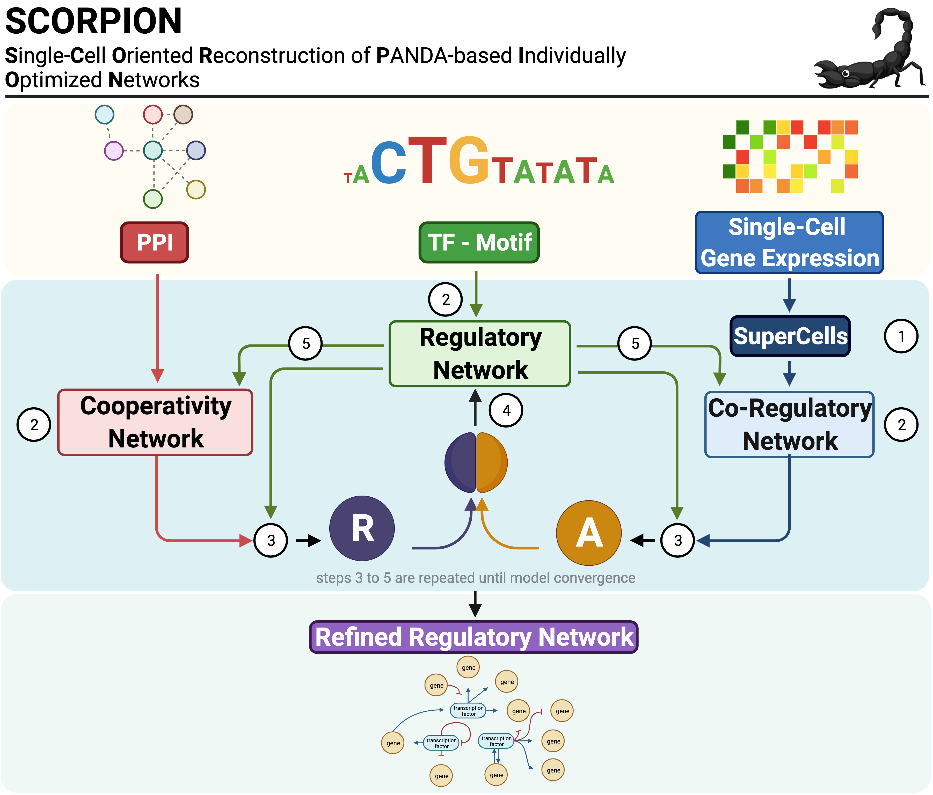
SCORPION (Single-Cell Oriented Reconstruction of PANDA Individually Optimized Gene Regulatory Networks) is an R package for constructing gene regulatory networks from single-cell and single-nucleus RNA sequencing data. The package addresses the sparsity inherent in single-cell expression data through coarse-graining, which aggregates similar cells to improve correlation structure detection. Network reconstruction is performed using the PANDA (Passing Attributes between Networks for Data Assimilation) message-passing algorithm, integrating transcription factor motifs, protein-protein interactions, and gene expression data. By using consistent baseline priors across samples, SCORPION produces comparable, fully-connected, weighted regulatory networks suitable for population-level analyses.
Installation
SCORPION is available on CRAN:
install.packages("SCORPION")
library(SCORPION)
To install the development version from GitHub:
devtools::install_github("kuijjerlab/SCORPION")
Quick Start
# Load example data
data(scorpionTest)
# Construct a single regulatory network
network <- scorpion(
  tfMotifs = scorpionTest$tf,
  gexMatrix = scorpionTest$gex,
  ppiNet = scorpionTest$ppi
)
# Construct networks stratified by cell groups
networks <- runSCORPION(
  gexMatrix = scorpionTest$gex,
  tfMotifs = scorpionTest$tf,
  ppiNet = scorpionTest$ppi,
  cellsMetadata = scorpionTest$metadata,
  groupBy = "region"
)
Example Data
The package includes scorpionTest, a dataset containing colorectal cancer single-cell RNA-seq data with the following components:
| Object | Type | Description |
|---|---|---|
gex |
dgCMatrix | Gene expression matrix (300 genes × 1,954 cells) |
tf |
data.frame | Transcription factor-target gene motif pairs from DoRothEA |
ppi |
data.frame | Protein-protein interaction network |
metadata |
data.frame | Cell-level annotations including donor, tissue region, and cell type |
Region codes: T = Tumor, B = Border (adjacent normal), N = Normal
data(scorpionTest)
str(scorpionTest)
List of 4
$ gex     :Formal class 'dgCMatrix' [package "Matrix"] with 6 slots
  ..@ Dim     : int [1:2] 300 1954
  ..@ Dimnames:List of 2
  .. ..$ : chr [1:300] "IGHM" "IGHG2" "IGLC3" ...
  .. ..$ : chr [1:1954] "P31-T_AAACGGGTCGGTTAAC" ...
$ tf      :'data.frame': 371738 obs. of  3 variables:
  ..$ source_genesymbol: chr [1:371738] "MYC" "SPI1" ...
  ..$ target_genesymbol: chr [1:371738] "TERT" "BGLAP" ...
  ..$ weight           : num [1:371738] 1 1 1 ...
$ ppi     :'data.frame': 4076 obs. of  3 variables:
  ..$ source_genesymbol: chr [1:4076] "ZIC1" "HES5" ...
  ..$ target_genesymbol: chr [1:4076] "ATOH1" "ATOH1" ...
  ..$ weight           : num [1:4076] 1 1 1 ...
$ metadata:'data.frame': 1954 obs. of  4 variables:
  ..$ cell_id  : chr [1:1954] "P31-T_AAACGGGTCGGTTAAC" ...
  ..$ donor    : chr [1:1954] "P31" "P31" ...
  ..$ region   : chr [1:1954] "T" "T" ...
  ..$ cell_type: Factor w/ 1 level "Epithelial": 1 1 ...
Core Functions
scorpion
Constructs a single gene regulatory network from a gene expression matrix using coarse-graining and the PANDA algorithm.
Usage:
result <- scorpion(
  tfMotifs = NULL,
  gexMatrix,
  ppiNet = NULL,
  computingEngine = "cpu",
  nCores = 1,
  gammaValue = 10,
  nPC = 25,
  assocMethod = "pearson",
  alphaValue = 0.1,
  hammingValue = 0.001,
  nIter = Inf,
  outNet = c("regNet", "coregNet", "coopNet"),
  zScaling = TRUE,
  showProgress = TRUE,
  randomizationMethod = "None",
  scaleByPresent = FALSE,
  filterExpr = FALSE
)
Parameters:
| Parameter | Description | Default |
|---|---|---|
tfMotifs |
Data frame with columns [TF, target gene, motif score]. Pass NULL for co-expression analysis only |
NULL |
gexMatrix |
Expression matrix with genes in rows and cells in columns | Required |
ppiNet |
Data frame with columns [protein1, protein2, interaction score]. Pass NULL to disable PPI integration |
NULL |
computingEngine |
Computation backend: cpu or gpu |
cpu |
nCores |
Number of processors for BLAS/MPI parallel computation | 1 |
gammaValue |
Coarse-graining level; ratio of cells to super-cells | 10 |
nPC |
Number of principal components for kNN network construction | 25 |
assocMethod |
Gene association method: pearson, spearman, or pcNet |
pearson |
alphaValue |
Weight of prior networks relative to expression data (0–1) | 0.1 |
hammingValue |
Convergence threshold based on Hamming distance | 0.001 |
nIter |
Maximum number of PANDA iterations before stopping | Inf |
outNet |
Networks to return: regNet, coregNet, and/or coopNet |
All three |
zScaling |
Return Z-score normalized edge weights; FALSE returns [0,1] scale |
TRUE |
showProgress |
Print progress messages during computation | TRUE |
randomizationMethod |
Randomization for null models: None, within.gene, or by.gene |
None |
scaleByPresent |
Scale correlations by percentage of cells with non-zero expression | FALSE |
filterExpr |
Remove genes with zero expression across all cells before inference | FALSE |
Return value:
A list containing:
| Component | Description |
|---|---|
regNet |
Regulatory network matrix (TFs × target genes) |
coregNet |
Co-regulation network matrix (genes × genes) |
coopNet |
TF cooperation network matrix (TFs × TFs) |
numGenes |
Number of genes in the network |
numTFs |
Number of transcription factors |
numEdges |
Total number of edges in the regulatory network |
runSCORPION
Constructs regulatory networks for multiple cell groups defined by metadata columns. This function wraps scorpion() to enable stratified network inference and returns results in a format suitable for comparative analysis.
Usage:
networks <- runSCORPION(
  gexMatrix,
  tfMotifs,
  ppiNet,
  cellsMetadata,
  groupBy,
  normalizeData = TRUE,
  removeBatchEffect = FALSE,
  batch = NULL,
  minCells = 30,
  ...
)
Parameters:
| Parameter | Description | Default |
|---|---|---|
gexMatrix |
Expression matrix with genes in rows and cells in columns | Required |
tfMotifs |
Data frame with columns [TF, target gene, motif score] | Required |
ppiNet |
Data frame with columns [protein1, protein2, interaction score] | Required |
cellsMetadata |
Data frame with cell-level metadata; must contain columns specified in groupBy |
Required |
groupBy |
Character vector of column name(s) in cellsMetadata for stratification |
Required |
normalizeData |
Apply log normalization to expression data before network inference | TRUE |
removeBatchEffect |
Perform batch effect correction before network inference | FALSE |
batch |
Factor or vector giving batch assignment for each cell; required if removeBatchEffect = TRUE |
NULL |
minCells |
Minimum number of cells required per group to build a network | 30 |
Additional parameters: All scorpion() parameters (computingEngine, nCores, gammaValue, nPC, assocMethod, alphaValue, hammingValue, nIter, outNet, zScaling, showProgress, randomizationMethod, scaleByPresent, filterExpr) can be passed to control network inference behavior. See scorpion() documentation above.
Return value:
A data frame in wide format where:
- Rows represent TF-target pairs
- Columns represent network identifiers (derived from
groupByvalues) - Values are edge weights from each network
Example output:
| tf | target | P31--T | P31--B | P31--N | P32--T | ... |
|---|---|---|---|---|---|---|
| AATF | ACKR1 | -0.326 | -0.337 | -0.344 | -0.298 | ... |
| ABL1 | ACKR1 | -0.340 | -0.339 | -0.351 | -0.312 | ... |
Examples:
# Stratify by tissue region
nets_by_region <- runSCORPION(
  gexMatrix = scorpionTest$gex,
  tfMotifs = scorpionTest$tf,
  ppiNet = scorpionTest$ppi,
  cellsMetadata = scorpionTest$metadata,
  groupBy = "region"
)
# Stratify by multiple variables
nets_by_donor_region <- runSCORPION(
  gexMatrix = scorpionTest$gex,
  tfMotifs = scorpionTest$tf,
  ppiNet = scorpionTest$ppi,
  cellsMetadata = scorpionTest$metadata,
  groupBy = c("donor", "region")
)
# With batch effect correction
nets_corrected <- runSCORPION(
  gexMatrix = scorpionTest$gex,
  tfMotifs = scorpionTest$tf,
  ppiNet = scorpionTest$ppi,
  cellsMetadata = scorpionTest$metadata,
  groupBy = "region",
  removeBatchEffect = TRUE,
  batch = scorpionTest$metadata$donor
)
Statistical Analysis
testEdges
Performs statistical testing on network edges to identify differential regulatory relationships between groups. The function supports single-sample tests, two-sample comparisons, and paired tests. All computations are fully vectorized for efficiency with large-scale datasets.
Usage:
results <- testEdges(
  networksDF,
  testType = c("single", "two.sample"),
  group1,
  group2 = NULL,
  paired = FALSE,
  alternative = "two.sided",
  padjustMethod = "BH",
  minLog2FC = 0,
  moderateVariance = TRUE,
  empiricalNull = TRUE,
  nCores = 1L,
  batchSize = NULL
)
Parameters:
| Parameter | Description | Default |
|---|---|---|
networksDF |
Output from runSCORPION() |
Required |
testType |
Test type: single (one-sample) or two.sample |
Required |
group1 |
Column names for the first (or only) group | Required |
group2 |
Column names for the second group (two-sample tests) | NULL |
paired |
Perform paired t-test; requires equal-length groups in matched order | FALSE |
alternative |
Alternative hypothesis: two.sided, greater, or less |
two.sided |
padjustMethod |
Multiple testing correction method (see p.adjust) |
BH |
minLog2FC |
Minimum absolute log2 fold change for inclusion (two-sample/paired only) | 0 |
moderateVariance |
Apply SAM-style variance moderation; adds median(SE) to denominator | TRUE |
empiricalNull |
Use Efron's empirical null (median/MAD) for p-value calibration | TRUE |
nCores |
Number of parallel workers. When >1, edges are split into batches processed via furrr::future_map_dfr. Requires furrr and future |
1 |
batchSize |
Rows per batch for parallel processing. NULL auto-calculates as ceiling(nrow(networksDF) / nCores). Only used when nCores > 1 |
NULL |
Return value:
A data frame containing:
| Column | Description |
|---|---|
tf, target |
TF-target pair identifiers |
meanEdge |
Mean edge weight (single-sample) |
meanGroup1, meanGroup2 |
Group means (two-sample) |
cohensD |
Cohen's d effect size (two-sample and paired tests) |
log2FoldChange |
Log2 fold change, Group1 − Group2 (two-sample) |
tStatistic |
t-statistic |
pValue |
Raw p-value |
pAdj |
Adjusted p-value |
Examples:
# Build networks stratified by donor and region
nets <- runSCORPION(
  gexMatrix = scorpionTest$gex,
  tfMotifs = scorpionTest$tf,
  ppiNet = scorpionTest$ppi,
  cellsMetadata = scorpionTest$metadata,
  groupBy = c("donor", "region")
)
# Define groups
tumor_nets <- grep("--T$", colnames(nets), value = TRUE)
normal_nets <- grep("--N$", colnames(nets), value = TRUE)
# Two-sample comparison: Tumor vs Normal
results <- testEdges(
  networksDF = nets,
  testType = "two.sample",
  group1 = tumor_nets,
  group2 = normal_nets
)
# Paired test for matched samples (same patient)
tumor_ordered <- c("P31--T", "P32--T", "P33--T")
normal_ordered <- c("P31--N", "P32--N", "P33--N")
results_paired <- testEdges(
  networksDF = nets,
  testType = "two.sample",
  group1 = tumor_ordered,
  group2 = normal_ordered,
  paired = TRUE
)
# Single-sample test: edges differing from zero
results_single <- testEdges(
  networksDF = nets,
  testType = "single",
  group1 = tumor_nets
)
regressEdges
Performs linear regression to identify edges with significant trends across ordered conditions. This is useful for studying disease progression or developmental trajectories.
Usage:
results <- regressEdges(
  networksDF,
  orderedGroups,
  padjustMethod = "BH",
  minMeanEdge = 0
)
Parameters:
| Parameter | Description | Default |
|---|---|---|
networksDF |
Output from runSCORPION() |
Required |
orderedGroups |
Named list of column name vectors; list order defines progression | Required |
padjustMethod |
Multiple testing correction method | BH |
minMeanEdge |
Minimum mean absolute edge weight for inclusion | 0 |
Return value:
A data frame containing:
| Column | Description |
|---|---|
tf, target |
TF-target pair identifiers |
slope |
Regression slope (change per condition step) |
intercept |
Regression intercept |
rSquared |
Coefficient of determination |
fStatistic |
F-statistic for the regression |
pValue |
Raw p-value |
pAdj |
Adjusted p-value |
meanEdge |
Overall mean edge weight |
mean<Condition> |
Mean edge weight for each condition |
Example:
# Define ordered progression: Normal → Border → Tumor
ordered_conditions <- list(
  Normal = grep("--N$", colnames(nets), value = TRUE),
  Border = grep("--B$", colnames(nets), value = TRUE),
  Tumor = grep("--T$", colnames(nets), value = TRUE)
)
# Identify edges with significant trends
results_reg <- regressEdges(
  networksDF = nets,
  orderedGroups = ordered_conditions
)
# Edges increasing along progression
increasing <- results_reg[results_reg$pAdj < 0.05 & results_reg$slope > 0, ]
# Edges decreasing along progression
decreasing <- results_reg[results_reg$pAdj < 0.05 & results_reg$slope < 0, ]
maEdges
Combines differential edge results from several independent studies into a
single meta-analytic estimate per TF-target pair, using either a fixed-effect
or DerSimonian-Laird random-effects model. Standard errors are recovered from
each study's log2FoldChange and pValue.
Usage:
results <- maEdges(
  edgesList,
  method = c("random", "fixed"),
  minStudies = 2
)
Parameters:
| Parameter | Description | Default |
|---|---|---|
edgesList |
List of testEdges() result data frames, one per study |
Required |
method |
Meta-analysis model: random or fixed |
random |
minStudies |
Minimum studies with valid values required per TF-target pair | 2 |
Return value:
A data frame containing:
| Column | Description |
|---|---|
tf, target |
TF-target pair identifiers |
k |
Number of contributing studies |
log2FoldChange |
Meta-analytic effect size |
se |
Standard error of the effect size |
ciLow, ciHigh |
95% confidence interval bounds |
zStatistic |
Z statistic |
pValue |
Raw p-value |
Q |
Cochran's Q heterogeneity statistic |
iSquared |
I-squared heterogeneity (%) |
tauSquared |
Between-study variance estimate |
pAdj |
Adjusted p-value (Benjamini-Hochberg) |
Example:
# Treat each patient's Tumor vs Normal comparison as a study
studyA <- testEdges(nets, "two.sample", group1 = "P31--T", group2 = "P31--N")
studyB <- testEdges(nets, "two.sample", group1 = "P32--T", group2 = "P32--N")
meta <- maEdges(list(studyA, studyB), method = "random")
Functional Enrichment
enrichEdges
Runs gene set enrichment analysis separately for each transcription factor,
ranking its target genes by a chosen edge-level statistic (e.g.
log2FoldChange) and testing enrichment with the multilevel fgsea algorithm.
TFs are processed in parallel.
Requires the fgsea package (Bioconductor):
BiocManager::install("fgsea")
Usage:
results <- enrichEdges(
  edgesDF,
  geneSets,
  numericValue,
  nCores = 3,
  seed = 1
)
Parameters:
| Parameter | Description | Default |
|---|---|---|
edgesDF |
Output from testEdges() with tf, target and numericValue columns |
Required |
geneSets |
Named list of gene sets | Required |
numericValue |
Name of the edgesDF column used as the ranking statistic |
Required |
nCores |
Number of parallel workers | 3 |
seed |
Random seed for the parallel enrichment calculations | 1 |
Return value:
A data frame containing:
| Column | Description |
|---|---|
tf |
Transcription factor |
geneSet |
Gene set identifier |
pValue |
Raw enrichment p-value |
pAdj |
Adjusted p-value (Benjamini-Hochberg) |
log2Err |
Expected log2 error of the p-value estimate |
ES |
Enrichment score |
NES |
Normalized enrichment score |
geneSetSize |
Number of set genes found among the targets |
Example:
res <- testEdges(
  networksDF = nets,
  testType = "two.sample",
  group1 = grep("--T$", colnames(nets), value = TRUE),
  group2 = grep("--N$", colnames(nets), value = TRUE)
)
geneSets <- list(
  SetA = c("ACKR1", "ACTA2"),
  SetB = c("ACTG2", "ADAMDEC1")
)
enr <- enrichEdges(
  edgesDF = res,
  geneSets = geneSets,
  numericValue = "log2FoldChange"
)
Visualization
circosEdges
Draws a circular (Circos) plot of differential TF–target links from a
testEdges() two-sample result. Genes are placed on their genomic coordinates;
link ribbons are colored continuously by log2FoldChange (diverging scale
centered at zero) and their thickness is proportional to -log10(pAdj). A
track of per-gene degree (the summed log2FoldChange of each gene's outgoing /
incoming links) is drawn as needles. Links are flagged known vs novel against
an optional a priori network, and gene labels are styled by role — TFs in
bold, targets in italics — showing only the top TFs/targets by absolute
degree to avoid overlap. By default only the main chromosomes are shown.
Requires the circlize package, and biomaRt when gene coordinates are
downloaded automatically:
install.packages("circlize")
BiocManager::install("biomaRt")
Usage:
circosEdges(
  edgesDF,
  species = "hsapiens_gene_ensembl",
  geneCoords = NULL,
  priorNet = NULL,
  geneSets = NULL,
  pAdjThreshold = 0.05,
  log2FCThreshold = 0,
  maxEdges = 500,
  colorBy = "log2FoldChange",
  linkColors = c("#2166AC", "#F7F7F7", "#B2182B"),
  lwdRange = c(0.5, 4),
  nmaxTF = 20,
  nmaxTarget = 20,
  knownColor = "grey60",
  novelColor = "#D95F02",
  geneSetColors = NULL,
  chromosomes = NULL,
  mainChromosomesOnly = TRUE,
  ensemblMirror = "www",
  transparency = 0.5,
  legend = TRUE
)
Parameters:
| Parameter | Description | Default |
|---|---|---|
edgesDF |
Output from testEdges() (two-sample or paired); needs tf, target, log2FoldChange, pAdj |
Required |
species |
Ensembl dataset for biomaRt when geneCoords is NULL (e.g. "mmusculus_gene_ensembl") |
"hsapiens_gene_ensembl" |
geneCoords |
Optional data frame (gene, chr, start, end) overriding the download for any source |
NULL |
priorNet |
Optional a priori TF–target network (first two columns); listed links are labeled known, others novel | NULL |
geneSets |
Optional GMT file path or named list of gene vectors to label around the circle | NULL |
pAdjThreshold |
Significance cutoff on pAdj (falls back to pValue) |
0.05 |
log2FCThreshold |
Minimum absolute log2FoldChange to draw a link |
0 |
maxEdges |
Cap on links drawn; keeps the most significant | 500 |
colorBy |
edgesDF column mapped to the continuous link color ramp |
"log2FoldChange" |
linkColors |
Length-3 low/mid/high color ramp (diverging for signed values) | blue–white–red |
lwdRange |
Min/max link line width; thickness scales with -log10(pAdj) |
c(0.5, 4) |
nmaxTF, nmaxTarget |
Number of TFs/targets to label, by largest absolute out-/in-degree (NULL/Inf = all) |
20, 20 |
knownColor, novelColor |
Border colors for known vs novel links | grey, orange |
geneSetColors |
Optional named colors for gene sets | auto |
chromosomes |
Optional subset/ordering of chromosomes shown | all present |
mainChromosomesOnly |
Drop unplaced scaffolds/contigs, keeping numbered chromosomes plus X, Y, MT | TRUE |
ensemblMirror |
biomaRt mirror: "www", "useast", "asia" |
"www" |
transparency |
Link transparency in [0, 1] (0 = opaque) |
0.5 |
legend |
Draw legends for effect size, novelty and gene sets | TRUE |
Return value:
Invisibly, a list with edges (plotted links annotated with coordinates and
novelty) and coords (the gene coordinate table with outDegree, inDegree
and total degree columns). Called for the side effect of drawing the plot.
Example:
# Two-sample comparison: Tumor vs Normal
res <- testEdges(
  networksDF = nets,
  testType = "two.sample",
  group1 = grep("--T$", colnames(nets), value = TRUE),
  group2 = grep("--N$", colnames(nets), value = TRUE)
)
# Human coordinates auto-downloaded from Ensembl,
# links flagged known/novel against a prior network,
# and hallmark gene sets labeled around the circle
circosEdges(
  edgesDF = res,
  species = "hsapiens_gene_ensembl",
  priorNet = scorpionTest$tf,
  geneSets = "hallmark.gmt"
)
# Offline / other species: supply your own coordinates
coords <- data.frame(
  gene = c("TF1", "GENE1"),
  chr = c("1", "2"),
  start = c(1000, 5000),
  end = c(2000, 6000)
)
circosEdges(res, geneCoords = coords)
Citation
If you use SCORPION in your research, please cite:
Osorio, D., Capasso, A., Eckhardt, S.G. et al. Population-level comparisons of gene regulatory networks modeled on high-throughput single-cell transcriptomics data. Nature Computational Science 4, 237–250 (2024). https://doi.org/10.1038/s43588-024-00597-5
Additional Resources
- Supplementary Materials: https://github.com/dosorio/SCORPION/
- Issue Tracker: https://github.com/kuijjerlab/SCORPION/issues
- CRAN Package Page: https://cran.r-project.org/package=SCORPION