Ten C++ functions are exposed by this package:
std::string rgb2hex(double r, double g, double b);
std::string rgba2hex(double r, double g, double b, double a);
std::string hsluv2hex(double h, double s, double l);
std::string hsluv2hex(double h, double s, double l, double alpha);
std::string hsv2hex(double h, double s, double v);
std::string hsv2hex(double h, double s, double v, double alpha);
std::string hsl2hex(double h, double s, double l);
std::string hsl2hex(double h, double s, double l, double alpha);
std::string hsi2hex(double h, double s, double i);
std::string hsi2hex(double h, double s, double i, double alpha);
r, g, b ∈ [0, 255] (red, green, blue)
a, alpha ∈ [0, 1] (opacity)
h ∈ [0, 360] (hue)
s,l,v,i ∈ [0, 100] (saturation, lightness, value, intensity)
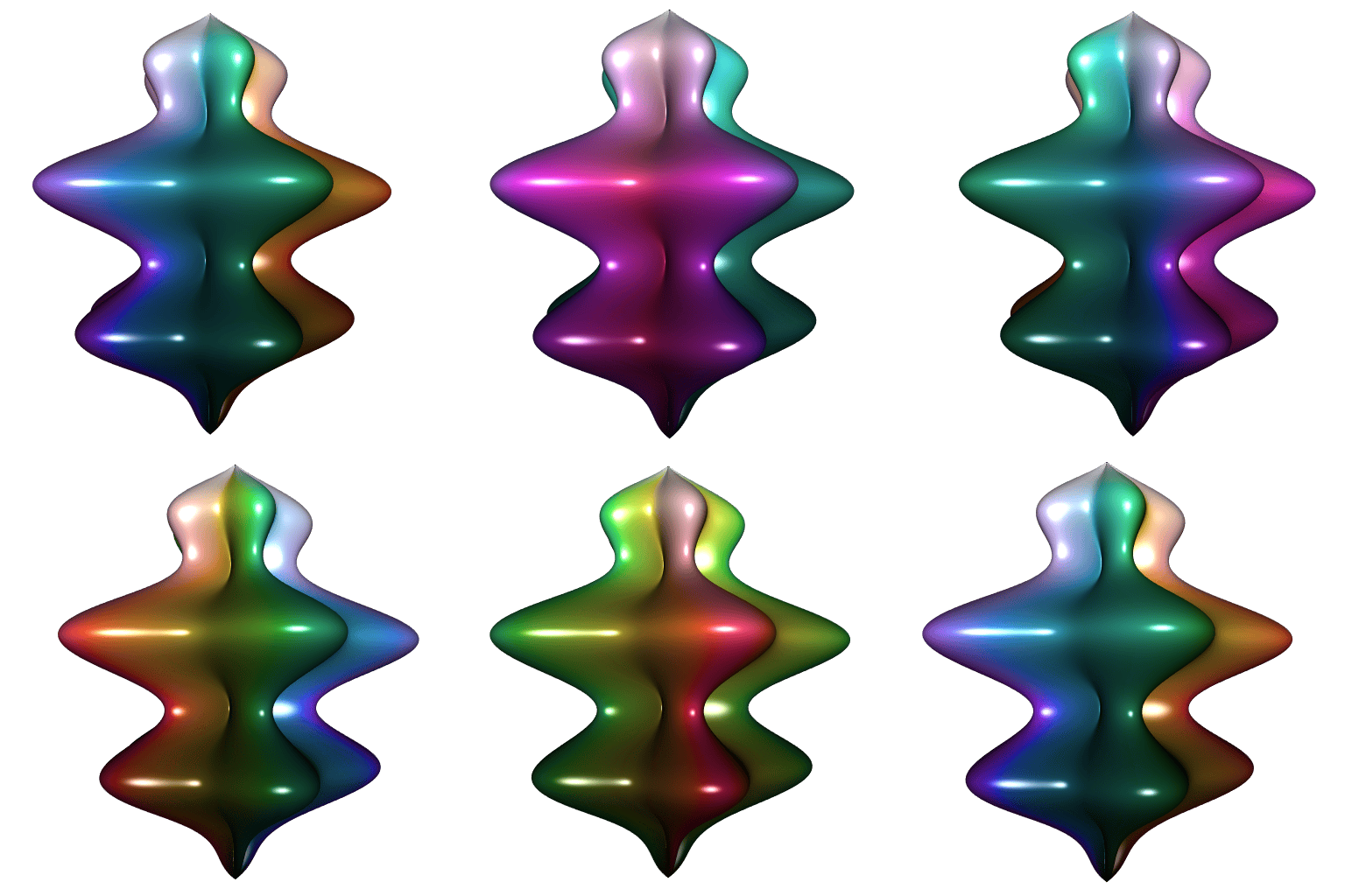
Usage in a package with Rcpp
The LinkingTo field in the DESCRIPTION file should look like
LinkingTo:
    Rcpp,
    RcppColors
Then, in your C++ file, you can call the above functions like this:
#include <RcppColors.h>
std::string mycolor = RcppColors::rgb2hex(0.0, 128.0, 255.0);
Color maps
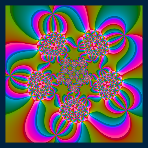
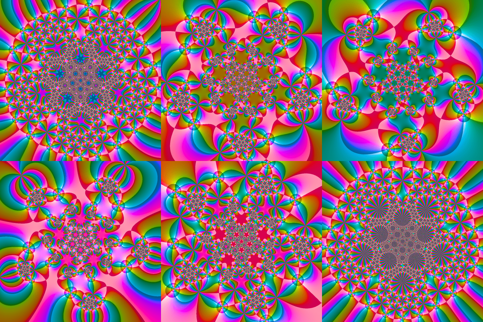
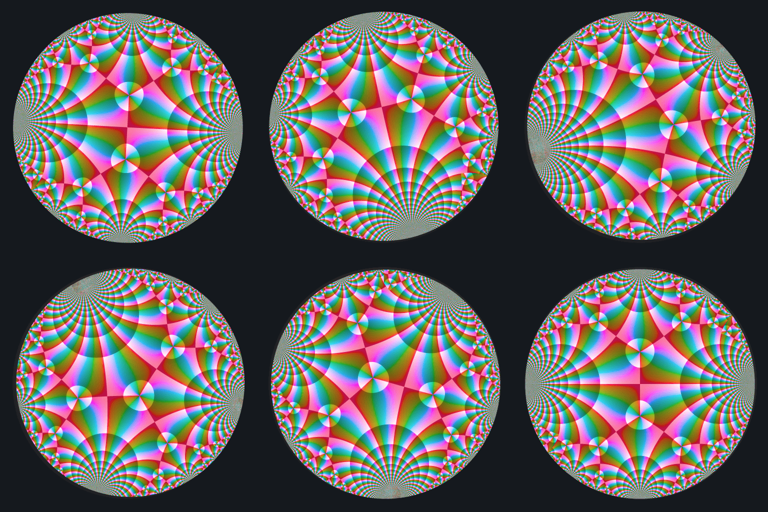
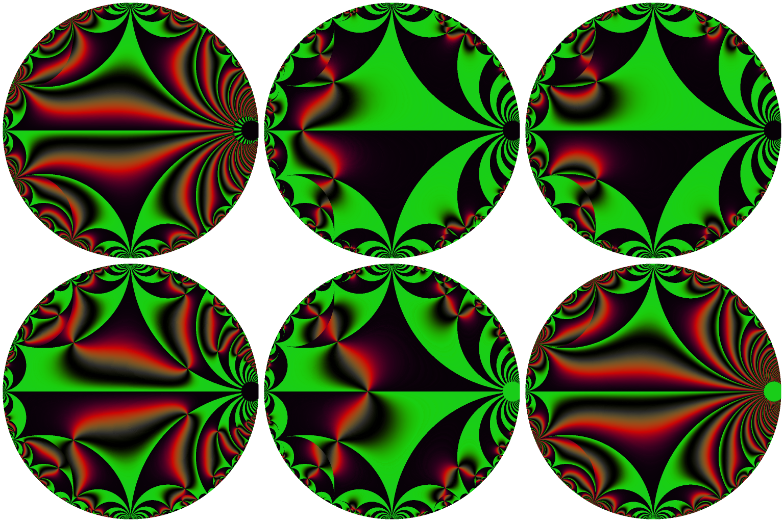
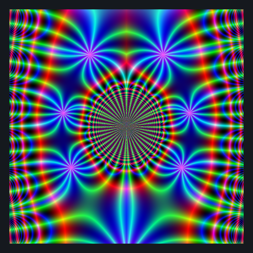
Fourteen color maps are available in R.
library(RcppColors)
library(Bessel)
x <- y <- seq(-4, 4, len = 1500)
# complex grid
W <- outer(y, x, function(x, y) complex(real = x, imaginary = y))
# computes Bessel values
Z <- matrix(BesselY(W, nu = 3), nrow = nrow(W), ncol = ncol(W))
# maps them to colors
image <- colorMap1(Z)
# plot
opar <- par(mar = c(0,0,0,0), bg = "#15191E")
plot(
  c(-100, 100), c(-100, 100), type = "n",
  xlab = "", ylab = "", axes = FALSE, asp = 1
)
rasterImage(image, -100, -100, 100, 100)
par(opar)
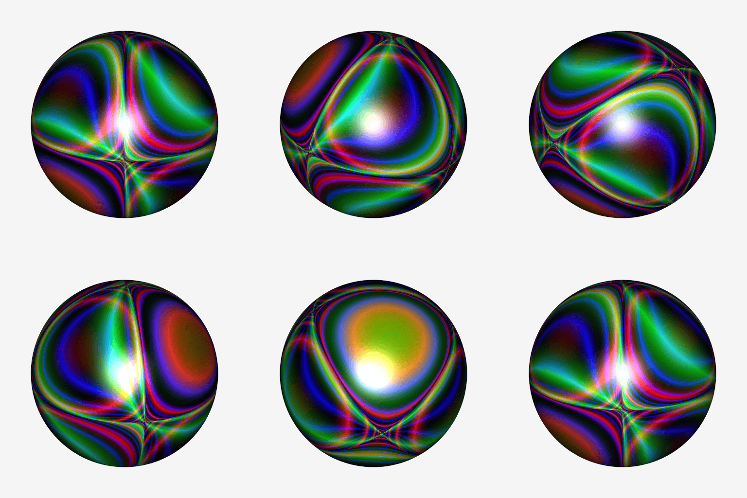
library(RcppColors)
library(Carlson)
library(rgl)
library(Rvcg)
mesh <- vcgSphere(subdivision = 8)
color <- apply(mesh$vb[-4L, ], 2L, function(xyz){
  if(sum(xyz == 0) >= 2){
    z <- NA_complex_
  }else{
    a <- xyz[1]
    b <- xyz[2]
    c <- xyz[3]
    z <- Carlson_RJ(a, b, c, 1i, 1e-5)
  }
  colorMap1(z)
})
mesh$material <- list(color = color)
open3d(windowRect = c(50, 50, 562, 562), zoom = 0.75)
bg3d("whitesmoke")
shade3d(mesh)
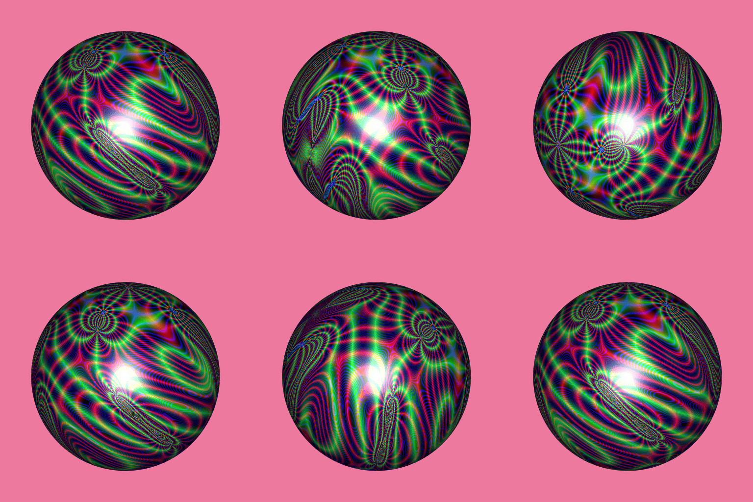
library(RcppColors)
library(jacobi)
library(rgl)
library(Rvcg)
mesh <- vcgSphere(subdivision = 8)
color <- apply(mesh$vb[-4L, ], 2L, function(xyz){
  a <- xyz[1]
  b <- xyz[2]
  c <- xyz[3]
  z <- wzeta(a + 1i* b, tau = (1i+c)/2)
  colorMap1(z)
})
mesh$material <- list(color = color)
open3d(windowRect = c(50, 50, 562, 562), zoom = 0.75)
bg3d("palevioletred2")
shade3d(mesh)
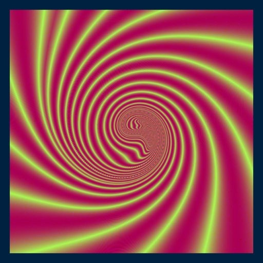
library(RcppColors)
ikeda <- Vectorize(function(x, y, tau0 = 0, gamma = 2.5){
  for(k in 1L:5L){
    tau <- tau0 - 6.0/(1.0 + x*x + y*y)
    newx <- 0.97 + gamma * (x*cos(tau) - y*sin(tau))
    y <- gamma * (x*sin(tau)+y*cos(tau))
    x <- newx
  }
  z <- complex(real = x, imaginary = y)
  colorMap1(z, reverse = c(TRUE, FALSE, FALSE))
})
x <- y <- seq(-3, 3, len = 3000)
image <- outer(y, x, function(x, y) ikeda(x, y))
opar <- par(mar = c(0,0,0,0), bg = "#002240")
plot(
  c(-100, 100), c(-100, 100), type = "n",
  xlab = "", ylab = "", axes = FALSE, asp = 1
)
rasterImage(image, -100, -100, 100, 100)
par(opar)
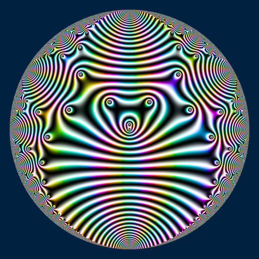
library(RcppColors)
library(jacobi)
f <- Vectorize(function(q){
  if(Mod(q) > 1  || (Im(q) == 0 && Re(q) <= 0)){
    z <- NA_complex_
  }else{
    z <- EisensteinE(6, q)
  }
  colorMap2(z, bkgcolor = "#002240")
})
x <- y <- seq(-1, 1, len = 2000)
image <- outer(y, x, function(x, y){
  f(complex(real = x, imaginary = y))
})
opar <- par(mar = c(0,0,0,0), bg = "#002240")
plot(
  c(-100, 100), c(-100, 100), type = "n",
  xlab = "", ylab = "", axes = FALSE, asp = 1
)
rasterImage(image, -100, -100, 100, 100)
par(opar)
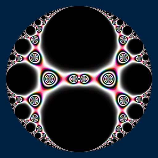
library(RcppColors)
library(jacobi)
f <- Vectorize(function(q){
  if(Mod(q) >= 1){
    NA_complex_
  }else{
    tau <- -1i * log(q) / pi
    if(Im(tau) <= 0){
      NA_complex_
    }else{
      kleinj(tau) / 1728
    }
  }
})
x <- y <- seq(-1, 1, len = 3000)
Z <- outer(y, x, function(x, y){
  f(complex(real = x, imaginary = y))
})
image <- colorMap2(1/Z, bkgcolor = "#002240", reverse = c(T,T,T))
opar <- par(mar = c(0,0,0,0), bg = "#002240")
plot(
  c(-100, 100), c(-100, 100), type = "n",
  xlab = "", ylab = "", axes = FALSE, asp = 1
)
rasterImage(image, -100, -100, 100, 100)
par(opar)
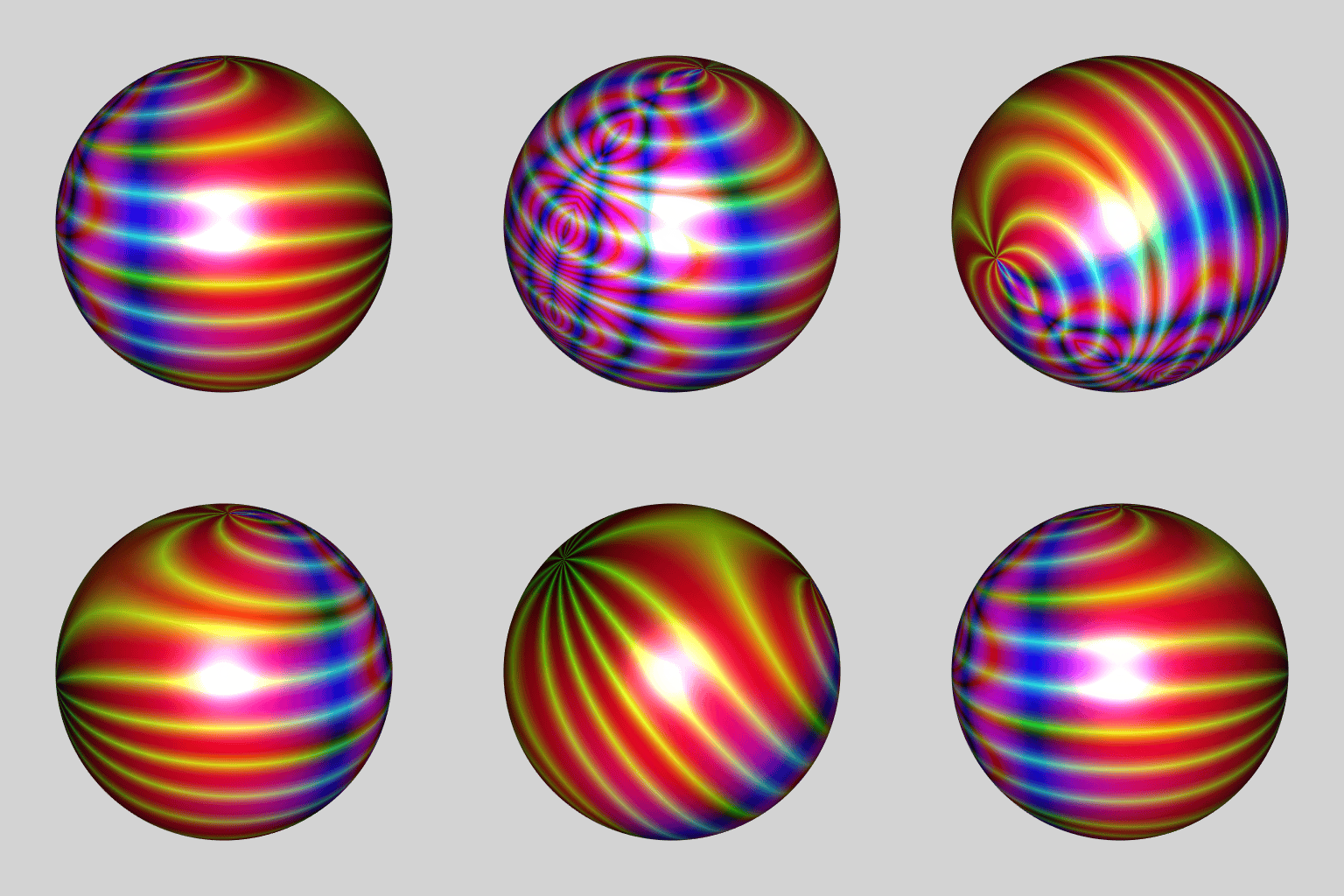
library(RcppColors)
library(jacobi)
library(rgl)
library(Rvcg)
library(pracma)
mesh <- vcgSphere(8)
sphcoords <- cart2sph(t(mesh$vb[-4L, ]))
theta <- sphcoords[, 1L] / pi
phi   <- sphcoords[, 2L] / pi * 2
Z <- wsigma(theta + 1i * phi, tau = 2+2i)
color <- colorMap1(Z, reverse = c(TRUE, FALSE, TRUE))
mesh$material <- list(color = color)
open3d(windowRect = c(50, 50, 562, 562), zoom = 0.75)
bg3d("lightgrey")
shade3d(mesh)
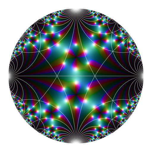
# Klein-Fibonacci map ####
library(jacobi)
library(RcppColors)
# the modified Cayley transformation
Phi <- function(z) (1i*z + 1) / (z + 1i)
PhiInv <- function(z) {
  1i + (2i*z) / (1i - z)
}
# background color
bkgcol <- "#ffffff"
# make the color mapping
f <- function(x, y) {
  z <- complex(real = x, imaginary = y)
  w <- PhiInv(z)
  ifelse(
    Mod(z) > 0.96,
    NA_complex_,
    ifelse(
      y < 0,
      -1/w, w
    )
  )
}
x <- seq(-1, 1, length.out = 2048)
y <- seq(-1, 1, length.out = 2048)
Z <- outer(x, y, f)
K <- kleinj(Z) / 1728
G <- K / (1 - K - K*K)
image <- colorMap4(G, bkgcolor = bkgcol)
# plot
opar <- par(mar = c(0,0,0,0), bg = bkgcol)
plot(
  c(-1, 1), c(-1, 1), type = "n",
  xlab = NA, ylab = NA, axes = FALSE, asp = 1
)
rasterImage(image, -1, -1, 1, 1)
# now we add the Dedekind tessellation (the white lines)
library(PlaneGeometry)
isInteger <- function(x) abs(x - floor(x)) < x * 1e-6
abline(h = 0, col = "white", lwd = 2)
N <- 150L
for(n in 1L:N) {
  if(isInteger(n/2) && ((n/2L) %% 2L == 1L)) {
    next
  }
  for(p in 1:n) {
    q <- sqrt(n*n - p*p + 4L)
    cases <- (isInteger(q) && isInteger(q/2) && (n %% 2L == 1L)) ||
      (isInteger(q) && isInteger(q/4) && (n %% 4L == 0L))
    if(cases) {
      circ <- Circle$new(center = c(q, p)/n, radius = 2/n)
      draw(circ, border = "white", lwd = 2)
      circ <- Circle$new(center = c(-q, p)/n, radius = 2/n)
      draw(circ, border = "white", lwd = 2)
      circ <- Circle$new(center = c(q, -p)/n, radius = 2/n)
      draw(circ, border = "white", lwd = 2)
      circ <- Circle$new(center = c(-q, -p)/n, radius = 2/n)
      draw(circ, border = "white", lwd = 2)
    }
  }
}
par(opar)
library(RcppColors)
library(jacobi)
f <- Vectorize(function(z){
  wsigma(z, omega = c(1, 0.25 + 1i))
})
x <- y <- seq(-5, 5, length.out = 512)
Z <- outer(y, x, function(x, y){
  f(complex(real = x, imaginary = y))
})
image <- colorMap5(Z, bkgcolor = "#002240")
opar <- par(mar = c(0,0,0,0), bg = "#002240")
plot(
  c(-100, 100), c(-100, 100), type = "n", xaxs="i", yaxs="i",
  xlab = NA, ylab = NA, axes = FALSE, asp = 1
)
rasterImage(image, -100, -100, 100, 100)
par(opar)