MultiModalR performs Bayesian mixture modeling for multimodal data. It detects subpopulations and assigns probabilistic memberships using two advanced Markov Chain Monte Carlo (MCMC) algorithms implemented in optimized C++:

Metropolis-Hastings within Gibbs Sampler for Gaussian Mixture Models - Fast and robust
Dirichlet-Multinomial (collapsed Gibbs) - Slower and rigorously robust

🎯 Features

🚀 Dual MCMC algorithms: Choose between Metropolis-Hastings (speed) or Dirichlet-Multinomial (robustness) depending on your data
🔍 Enhanced Mode Detection: Height-aware peak detection with four bandwidth methods
📊 Bayesian Probability Assignment: Soft assignment with probability estimates
🎪 Subpopulation Detection: Automatic detection of multimodal components
⚡ Parallel Processing: Built-in multi-core computation
✅ Validation Tools: Built-in plotting and validation functions
🔄 Flexible Input: Works with various data structures
⚙️ Optimized C++ Core: Blazing fast MCMC sampling with RcppArmadillo

📋 Prerequisites

R Package Dependencies

Rcpp, RcppArmadillo, dplyr, furrr, future

System Requirements

R ≥ 4.0
Multiple CPU cores for parallel processing

💾 Installation

devtools::install_github("DijoG/MultiModalR")

🚀 Quick Start Example

library(MultiModalR)
# Load data
df <- MultiModalR::multimodal_dummy
# Run analysis with default settings
results <- fuss_PARALLEL_mcmc(
  data = df,
  varCLASS = "Category",
  varY = "Value",
  varID = "ID"
)
# View results summary
summary(results)

⚙️ Parameters

MultiModalR::fuss_PARALLEL_mcmc(
  data = df,                  # 📦 -> required
  varCLASS = "Category",      # 🏷️ -> required
  varY = "Value",             # 📈 -> required
  varID = "ID",               # 🆔 -> required
  method = "sj-dpi",          # 📏 /default
  within = 1,                 # 🎯 /default
  maxNGROUP = 5,              # 🔢 /default
  out_dir = ".../output",     # 💾 -> optional 
  n_workers = 3,              # ⚡ /default
  n_iter = NULL,              # 🔄 /default
  burnin = NULL,              # 🔥 /default
  proposal_sd = 0.15,         # 📊 /default
  sj_adjust = 0.5,            # ⚖️ /default
  mcmc_method = "metropolis", # 🧮 /default
  dirichlet_alpha = 2.0       # 🎲 /default
)

📚 Detailed Example

Data

library(MultiModalR)
# Load the built-in dataset
df <- MultiModalR::multimodal_dummy
# View the data structure
head(df)
str(df)

Data Visualization

library(ggplot2)
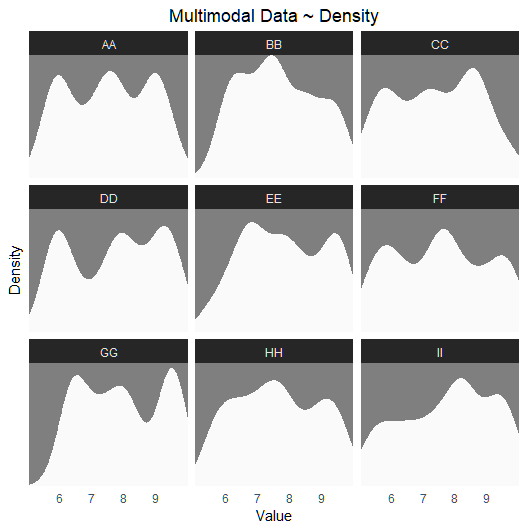
# Plot 01 ~ subpopulations/subgroups not shown
ggplot(df, aes(x = Value)) +
  geom_density(color = NA, fill = "grey98", adjust = .8) +
  facet_wrap(~Category) +
  theme_dark() +
  labs(title = "Multimodal Data ~ Density",
       x = "Value", y = "Density") +
  scale_y_continuous(expand = expansion(mult = c(0, 0))) +
  scale_x_continuous(expand = expansion(mult = c(0, 0))) +
  theme(legend.position = "top",
        axis.text.y = element_blank(),
        axis.ticks = element_blank(),
        panel.grid.major = element_blank(), panel.grid.minor = element_blank(),
        plot.title = element_text(hjust = .5))

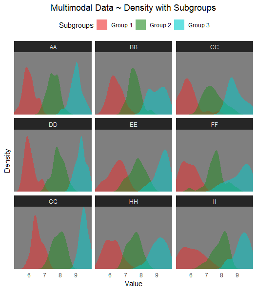
# Plot 02 ~ subgroups shown
ggplot(df, aes(x = Value, fill = Subpopulation)) +
  geom_density(alpha = 0.5, color = NA) +
  scale_fill_manual(values = c("firebrick2", "forestgreen", "cyan3"),
                     name = "Subgroups") +
  facet_wrap(~Category) +
  theme_dark() +
  labs(title = "Multimodal Data ~ Density with Subgroups",
       x = "Value", y = "Density") +
  scale_y_continuous(expand = expansion(mult = c(0, 0))) +
  scale_x_continuous(expand = expansion(mult = c(0, 0))) +
  theme(legend.position = "top",
        legend.key = element_rect(fill = "transparent", color = NA),
        axis.text.y = element_blank(),
        axis.ticks = element_blank(),
        panel.grid.major = element_blank(), panel.grid.minor = element_blank(),
        plot.title = element_text(hjust = .5)) +
  guides(fill = guide_legend(override.aes = list(alpha = .6)))

Parallel Processing Setup

# Configure parallel processing
cores <- 3

Running Analysis

# Dirichlet MCMC
MultiModalR::fuss_PARALLEL_mcmc(
  data = df,
  varCLASS = "Category",
  varY = "Value",
  varID = "ID",
  out_dir = "D:/MultiModalR/test",
  n_workers = cores,
  mcmc_method = "dirichlet"
)
tictoc::toc()
# Processing time: 5.19 sec (3 cores) ~ 91.4% overall accuracy
# -- OR (recommended default) -->
# Metropolis-Hastings within Gibbs Sampler for Gaussian Mixture Models 
MultiModalR::fuss_PARALLEL_mcmc(
  data = df,
  varCLASS = "Category",
  varY = "Value",
  varID = "ID",
  out_dir = "D:/MultiModalR/test",
  n_workers = cores
)
tictoc::toc()
# Processing time: 3.18 sec (3 cores) ~ 92% overall accuracy

Output

The function generates:

Data CSV files: Original data with assigned subgroups and probabilities

A Data CSV file consists of the following fields (maxNGROUP = 5):

y: Original/observed value
Group: Original/observed subgroup
Group_1: Predicted belonging probability to
Group_2: Predicted belonging probability to
Group_3: Predicted belonging probability to
Group_4: Predicted belonging probability to
Group_5: Predicted belonging probability to
Assigned_Group: Assigned/predicted subgroup
Min_Assigned: Minimum value of the assigned/predicted range
Max_Assigned: Maximum value of the assigned/predicted range
Mean_Assigned: Mean value of the assigned/predicted range
Mode_Assigned: Mode of the assigned/predicted range
Main_Class: Category/main group/class

Validation Visualization

# Validate subgroup assignments
MultiModalR::plot_VALIDATION(
  "D:/MultiModalR/test",
  df,
  subpop_col = "Subpopulation",
  value_col = "Value",
  id_col = "ID")

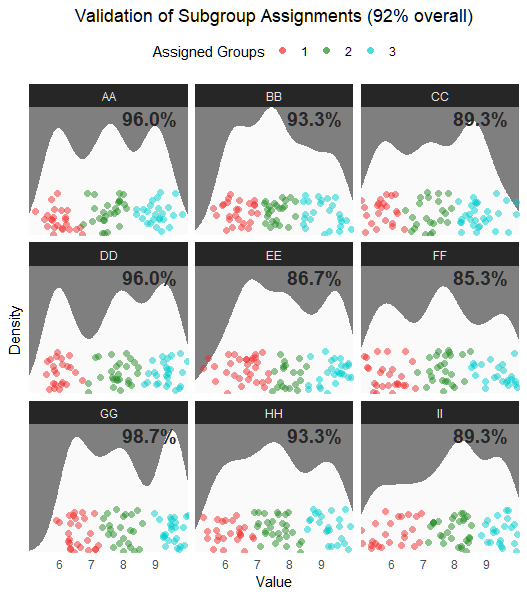
Validation results show accurate subgroup assignments across categories.

Generate Custom Data

You can also generate custom multimodal data with different parameters:

# Generate custom dataset
custom_data <- MultiModalR::create_multimodal_dummy(
  seed = 12,
  n_categories = 6,
  n_per_group = 30,
  n_subgroups = 4
)

Happy multimoda(e)ling! 🏔️️ 📊 🎯

📝 Citation

If you use MultiModalR in your research, please cite the original paper: after publication