The formation and evolution of galaxies has been a central concern of cosmology since E. P. Hubble (1929) demonstrated that spiral nebulae are external stellar systems of size comparable to the Milky Way. Ideas about the formation of galaxies have ranged from the monolithic collapse of giant gas clouds (O. J. Eggen et al. 1962) to assembly through the merger of numerous protogalactic fragments (L. Searle & R. Zinn 1978). With the launch of JWST, we now have the opportunity to directly observe the assembly of galaxies at early epochs, providing a direct test of these ideas.
In Lambda cold dark matter (ΛCDM), galaxies form in dark matter halos that originate from primordial density fluctuations that start small and grow gradually (D. N. Schramm 1992; P. J. E. Peebles 1993). Massive halos, and the galaxies that they contain, assemble from the merger of smaller halos (R. H. Wechsler & J. L. Tinker 2018). This hierarchical formation of structure is often depicted as a merger tree (R. S. Somerville & T. S. Kolatt 1999). The objects that are giant galaxies today are the products of the assembly of many protogalactic fragments.
There are two basic effects in play: (i) the assembly of mass and (ii) the emergence of an observable, luminous galaxy through the accretion of gas and its conversion into stars. The timeline of mass assembly (i) is well quantified by N-body simulations (G. De Lucia et al. 2006; C. Srisawat et al. 2013). The second step is highly uncertain, depending on many aspects of gas physics and star formation. However, the luminosity of an individual galaxy cannot outpace its assembly rate (T. Naab et al. 2009; C. Nipoti et al. 2009; A. van der Wel et al. 2009). Observations of the luminosities of galaxies thus test the predicted formation history.
We describe galaxy formation models in Section 2. Constraints on the evolution of high-redshift galaxies predating the launch of JWST are discussed in Section 3, and new insights from JWST data are examined in Section 4. Complementary constraints from kinematic observations are discussed in Section 5. Taken together, the data indicate that structure formed in the early Universe at an accelerated pace relative to the predictions of ΛCDM (Section 6). This result had been anticipated well in advance of the observations (R. H. Sanders 1998; S. S. McGaugh 2015), as discussed in Section 7. Section 8 provides a succinct summary. We adopt a vanilla ΛCDM Universe with Ωm = 0.3, ΩΛ = 0.7, and H0 = 70 km s−1 Mpc−1 for cosmology-dependent quantities.
It is important to have at least two distinct hypotheses to compare and contrast, so we consider both monolithic and hierarchical galaxy formation models. The passive evolution of a monolithic galaxy that forms early is motivated by traditional inferences about the evolutionary history of giant ellipticals (C. Chiosi & G. Carraro 2002; D. Thomas et al. 2005; J. N. Bregman et al. 2006; A. Renzini 2006; J. Schombert & K. Rakos 2009; J. M. Schombert 2016). In contrast, hierarchical galaxy formation is expected in ΛCDM (S. D. M. White & C. S. Frenk 1991), with testable predictions provided by both semianalytic galaxy formation models (SAMs) and hydrodynamical simulations. Though something of a straw man on its own, the monolithic case is useful as a proxy for the predictions (R. H. Sanders 1998) of modified Newtonian dynamics (MOND; M. Milgrom 1983).
2.1. Hierarchical ΛCDM Models
Hierarchical galaxy formation in ΛCDM is a combination of in situ star formation in the largest of many progenitors and ex situ growth via merging (H. J. Mo et al. 1998; B. M. B. Henriques et al. 2015; V. Rodriguez-Gomez et al. 2016; D. Angles-Alcazar et al. 2017; P. Behroozi & J. Silk 2018). The largest galaxies are predicted to form latest, as they take the longest to assemble. That large galaxies are observed to contain the oldest stars (J. N. Bregman et al. 2006; J. M. Schombert 2016) may thus seem like a contradiction, but it may simply mean that many of the stars formed in protogalaxies at early times prior to them merging into the final giant galaxy (G. De Lucia et al. 2006; A. Cattaneo et al. 2008; C. Nipoti et al. 2009; A. van der Wel et al. 2009). We thus expect to see many small precursor galaxies at high redshift for every modern giant (A. B. Newman et al. 2012; C. J. Conselice et al. 2022).
There are many papers in the literature discussing the evolution of galaxies, including theoretical works that attempt to predict how observable galaxies are associated with their parent dark matter halos. While important details vary from model to model (A. Knebe et al. 2015), the basic prediction of the hierarchical buildup of mass is common to all, as it is fundamental to the ΛCDM structure formation paradigm. This is well documented by many simulations, for example, the IllustrisTNG suite of magnetohydrodynamical simulations (F. Marinacci et al. 2018; J. P. Naiman et al. 2018; D. Nelson et al. 2018; A. Pillepich et al. 2018; V. Springel et al. 2018).
Figure 1 illustrates hierarchical galaxy formation as realized in the high-resolution TNG50 simulation (D. Nelson et al. 2019; A. Pillepich et al. 2019). The merger tree of one model galaxy (subhalo 6 of TNG50-1) is shown. Early, high-redshift epochs are dominated by mergers, a feature that is common to all galaxies in the hierarchical formation scenario. There is in general a great diversity of merger tree morphologies, with some continuing to experience significant mergers up to the present time. The illustrated example experiences its last merger and quenches relatively early (z ∼ 1), but the buildup of stellar mass in its largest progenitor follows the typical evolutionary track fairly closely, being only a little ahead of the median (V. Rodriguez-Gomez et al. 2016) at z ≈ 1.
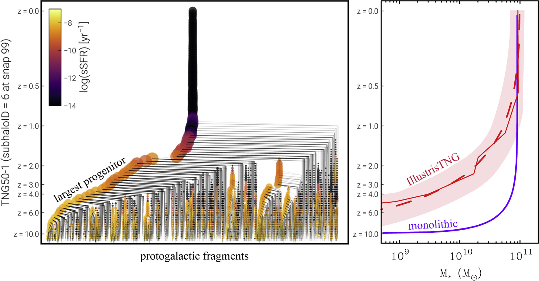
Figure 1. A merger tree for a model galaxy from the TNG50-1 simulation (D. Nelson et al. 2019; A. Pillepich et al. 2019; left panel) selected to have M* ≈ 9 × 10¹⁰ M☉ at z = 0, i.e., the stellar mass of a local L* early-type galaxy (S. P. Driver et al. 2022). Mass assembles hierarchically, starting from small halos at high redshift (bottom edge) with the largest progenitor traced along the left edge of the merger tree. The size of the symbol is proportional to the halo mass, and the color bar illustrates the specific star formation rate. The growth of the stellar mass of the largest progenitor is shown in the right panel. This example (jagged line) is close to the median (dashed line) of comparable-mass objects (V. Rodriguez-Gomez et al. 2016) and within the range of the scatter (the shaded band shows the 16th–84th percentiles). A monolithic model that forms at zf = 10 and evolves with an exponentially declining star formation rate (Equation (1)) with τ = 1 Gyr (purple line) is shown for comparison.
Download figure:
Standard image High-resolution imageA fundamental aspect of hierarchical galaxy formation is that a massive galaxy at z = 0 is the sum of many parts. As we look to high redshift, we do not expect to see an early version of the modern galaxy but rather its many precursor components. There is no single entity whose evolution we can trace. The closest thing to that is the largest progenitor, which takes time to assemble. For example, the typical L* galaxy in the Illustris simulation (V. Rodriguez-Gomez et al. 2016) takes about half a Hubble time (until z ≈ 0.7) to assemble half of its stars (Figure 1). This is why the observation of massive (M* > 1010 M☉) galaxies at z > 6 is surprising; such objects should be rare occurrences because there has not yet been sufficient time to assemble large objects from the many contributing protogalactic fragments (Figure 1).
Simulated galaxy stellar mass functions are in tolerable agreement with the data for z ≤ 2 (S. Genel et al. 2014; M. Furlong et al. 2015). Above this redshift, they start to diverge from the data in the sense that there are more bright, high-mass galaxies than expected (J. R. Franck & S. S. McGaugh 2017), with the discrepancy becoming clear at z > 4 (C. L. Steinhardt et al. 2016). From 6 < z < 10, there is a pronounced excess in the number of galaxies with M* ≈ 1010 M☉ over that predicted (S. S. McGaugh 2024). JWST observations extend this excess to even higher redshift (Section 4). We will discuss possible paths to understanding this in Section 6 after exploring the evidence.
2.2. Monolithic Models
An important touchstone in galaxy evolution is the case of the passive evolution of a monolithic island Universe (O. J. Eggen et al. 1962). The assumption implicit in this hypothesis is that practically all of the mass currently in a galaxy has always been part of it; it evolves as a closed box since a formation redshift zf . This provides a convenient picture but is an unrealistic oversimplification. Galaxy-mass balls of gas do not magically appear in the early Universe; mass must assemble from the initial condition of a nearly homogeneous early Universe (Planck Collaboration et al. 2020). This picture nevertheless provides a useful null hypothesis and a starting point for more realistic models that assemble mass rapidly if not instantaneously (C. Chiosi & G. Carraro 2002).
The growth of the stellar mass of a monolithic galaxy is determined by its star formation history. A common prescription for the passive evolution of a predominantly old stellar population like that of a typical elliptical galaxy (J. N. Bregman et al. 2006; K. Rakos et al. 2008; J. Schombert & K. Rakos 2009; J. M. Schombert 2016) is an exponentially declining star formation history:
Here, ψ0 is a star formation rate that sets the scale that leads to a final mass , and
where ti is the time after the Big Bang when star formation begins that we equate to the redshift of galaxy formation zf and τ is the timescale over which star formation activity fades. A population can be said to be passively evolving if this timescale is much shorter than a Hubble time so that most of the stars form in the early Universe and evolve passively thereafter. The stellar mass increases as
With this prescription for the buildup of stellar mass M*(t) and the time–redshift relation of vanilla ΛCDM, the luminosity evolution L(z) can be calculated using the methods of stellar population synthesis (A. Renzini 2006).
An exponential model with τ = 1 Gyr and a formation redshift zf
= 10 (ti
= 464 Myr for vanilla ΛCDM) forms half of its stellar mass by z = 5 (J. R. Franck & S. S. McGaugh 2017). This provides a baseline against which to compare other models (Figure 1). To relate light to mass, we adopt an empirical calibration of this model by equating the final mass to the characteristic stellar mass
of the Schechter fit to local early-type galaxies (S. P. Driver et al. 2022) and by matching the corresponding luminosity L* to the characteristic apparent magnitude m* of cluster galaxies at z ≈ 1 (C. L. Mancone et al. 2010). This data-informed choice of the mass-to-light ratio is within the range expected for the stellar population models built by J. R. Franck & S. S. McGaugh (2017): evolutionary theory and data agree at the expected level.
To improve on the exponential model without adding much complexity, we also consider a generalization that allows for a finite ramp-up of star formation before it quenches. D. D. Kelson et al. (2016) show that stochastic star formation leads to an average linear ramp-up in the star formation rate ψ ∼ t as galaxies accrete gas. This will quickly build up stellar mass as M* ∼ t2. This process is more monolithic than hierarchical, as it envisions in situ star formation from gas accretion onto a single object. Indeed, star formation must quench rapidly in order not to overproduce stellar mass. Regardless of the precise mechanism by which quenching occurs (Y. Peng et al. 2015; L. C. Kimmig et al. 2023), an obvious choice to model it is an exponential attenuation with a short e-folding time. Combining this with an initially linear ramp-up gives
This is only a slight modification to the traditional exponential star formation history described above, providing it with a more realistic initial condition. In principle, we could consider separate timescales for the ramp-up of star formation and its quenching and could also insert a time delay for the commencement of quenching. We eschew these details for now as unnecessary complications, as we seek only to quantify the approximate timescales relevant to explaining observations of massive galaxies at high redshift. We thus restrict ourselves to the two timescales ti and τ that are built into the definition of u (Equation (2)).
Integrating Equation (4), the stellar mass grows as
where is the final stellar mass. While no individual galaxy will have exactly this star formation history, Equation (5) provides a simple way to describe the formation and quenching timescales that characterize a population of galaxies as represented by the typical Schechter function L* galaxy and its corresponding mass
.
2.3. MOND Galaxy Formation Models
MOND has been very successful as a theory of galaxy dynamics (R. H. Sanders & S. S. McGaugh 2002; B. Famaey & S. S. McGaugh 2012; I. Banik & H. Zhao 2022) but has no completely satisfactory cosmology (B. Famaey & S. S. McGaugh 2012; N. Wittenburg et al. 2023). Perhaps the most successful attempt to combine MOND and general relativity to date is the aether scalar tensor (AeST) theory of C. Skordis & T. Złosnik (2019). AeST has been shown to fit the power spectrum of both the cosmic microwave background and galaxies at low redshift (C. Skordis & T. Złośnik 2021), but many details of the theory remain to be explored. One possible shortcoming is an apparent tension between the parameters required to explain the data at small, intermediate, and large scales (T. Mistele et al. 2023).
While the deeper theory remains unknown, we know that the Universe is expanding and that MOND often works to describe the dynamics of objects within it. In what follows, we consider what happens to a region within the expanding Universe that is subject to the MOND force law (R. H. Sanders 1998, 2008).
MOND is inherently nonlinear. A growth factor of ∼105 from z = 1090 to z = 0 is achieved through nonlinear growth (A. Nusser 2002; A. Knebe & B. K. Gibson 2004; C. Llinares et al. 2008) rather than linear growth with cold dark matter. Calculating the nonlinear growth of structure in MOND is a nontrivial problem (R. H. Sanders 1998; R. H. Sanders 2001; S. Stachniewicz & M. Kutschera 2001; A. Nusser 2002; S. S. McGaugh 2004; C. Llinares et al. 2008; M. Feix 2016; N. Wittenburg et al. 2020), and considerable work remains to be done. Nevertheless, a common feature of these analyses is a period of rapid structure formation. Indeed, this seems unavoidable when considering a MONDian region within an expanding background.
R. H. Sanders (1998) considered spherical regions in the MOND regime of low accelerations in an expanding Universe. After first showing that the usual early Universe results (e.g., Big Bang nucleosynthesis) are retained, R. H. Sanders (1998) showed that there is a characteristic length scale rc below which MOND dynamics should apply. The value of rc grows with time, with small regions entering the MOND regime first and larger ones later in a hierarchical sequence, albeit one greatly accelerated relative to ΛCDM. On scales larger than rc , the Universe remains homogeneous and isotropic, so the conventional Friedmann equation may continue to apply. On scales smaller than rc , the region becomes detached from the Hubble expansion and is destined to recollapse under its own gravity. This process is inevitably inefficient: not all regions of the Universe will be neat spheres that are cleanly in the MOND regime. Those that are must necessarily collapse rapidly, so there should be a portion of the galaxy population that forms early.
The governing equation for an initially expanding spherical region in the MOND regime (J. E. Felten 1984; R. H. Sanders 1998) is
where r0 is the comoving radius of the spherical region, ri
and are the initial radius and expansion velocity thereof, ρb
is the baryonic mass density, and a0 = 1.2 × 10⁻¹⁰ m s−2 (K. G. Begeman et al. 1991; S. S. McGaugh et al. 2016). The introduction of the dimensional constant a0 makes the problem scale-dependent (J. E. Felten 1984), so the initial conditions matter. Fortunately, ri
and
have an obvious interpretation: since this growth can only commence after radiation releases its grip on the baryons, the initial velocity is simply the cosmic expansion rate at that time, while the initial radius specifies the mass of the object. The precise redshift when this occurs is sensitive to the cosmology (R. H. Sanders 1998) but happens early enough (z ≳ 200) that the net result for galaxy-mass objects is not particularly sensitive to the initial conditions: the start time is small compared to the subsequent evolution.
A region that evolves according to Equation (6) reaches a maximum radius and recollapses on a timescale comparable to that of the initial expansion (Figure 2). In a pure MOND Universe, such a region is destined to recollapse (J. E. Felten 1984) irrespective of its initial density (Equation (6)). Small regions naturally collapse faster than large ones, so the process is inherently hierarchical, but the timescale is greatly accelerated relative to the linear case. The mass of the top hat sets the timescale for decoupling from the Hubble flow (R. H. Sanders 1998) and recollapse (S. Stachniewicz & M. Kutschera 2001). Hydrodynamics is important at the scale of globular clusters, which briefly delays their collapse, but is less important at galaxy scales (S. Stachniewicz & M. Kutschera 2001).
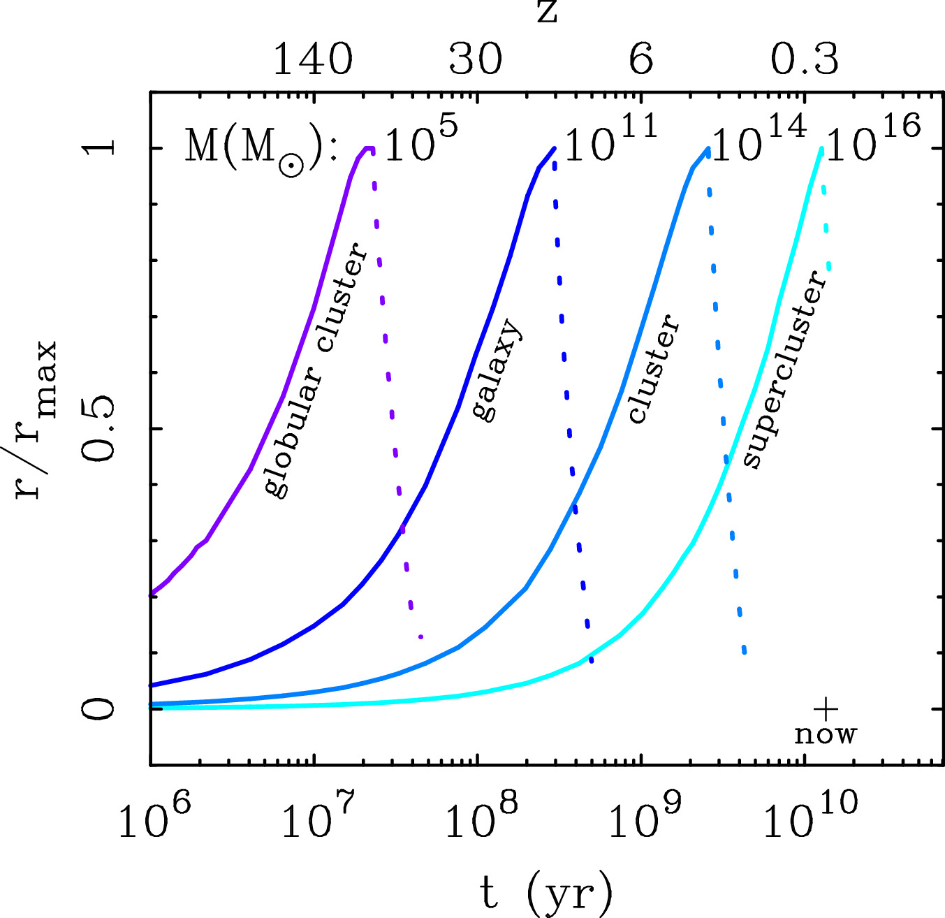
Figure 2. The expansion (solid lines) and collapse (dotted lines) of spherical regions of various baryonic masses in MOND as a function of time (R. H. Sanders 1998). Globular clusters collapse first and form early. Large galaxies reach maximum expansion after ∼3 × 10⁸ yr; rich clusters of galaxies do so after ∼3 × 10⁹ yr. Laniakea (R. B. Tully et al. 2014) and Ho’oleilana (R. B. Tully et al. 2023) may be examples of vast structures near turnaround today. The redshift scale on the top axis assumes vanilla ΛCDM for reference, but the time–redshift relation may differ in MOND.
Download figure:
Standard image High-resolution imageGlobular-cluster-mass (∼105 M☉) objects collapse very quickly, in the first 100 Myr (S. Stachniewicz & M. Kutschera 2001). This is so fast that they will have ages that are practically indistinguishable from that of the Universe itself (J. M. Ying et al. 2023). Massive (∼1011 M☉) galaxies reach maximum expansion around 300 Myr (R. H. Sanders 1998), with collapse happening on a similar timescale (S. Stachniewicz & M. Kutschera 2001). N. Wittenburg et al. (2020) considered slightly lower-mass objects and found that the initial spheres collapse to form a thin, rotating disk after ∼500 Myr. This is the epoch of galaxy formation in MOND (see also R. H. Sanders 2001; S. S. McGaugh 2004; C. Llinares et al. 2008; R. H. Sanders 2008). Thus, even though structure formation in MOND remains intrinsically hierarchical, the timescales are so short that the monolithic models described in Section 2.2 provide a reasonable first approximation.
The discussion above outlines two distinct hypotheses: hierarchical and monolithic galaxy formation. Hierarchical galaxy formation is expected in ΛCDM, while monolithic galaxy formation is a first approximation to the accelerated structure formation expected in MOND. We can test these hypotheses by observing the evolutionary development of galaxies over a wide range of redshifts. In this paper, we focus on tracing the growth of galaxy stellar mass utilizing photometric observations over the range 0 < z < 15. We also consider the constraints on dynamical mass provided by kinematic observations over the past 11 Gyr. These complimentary lines of evidence provide a consistent picture in which a significant population of massive galaxies formed remarkably early.
As we look to high redshift, the first objects we see are always the brightest beacons that have been lit at that time. We must therefore take care to consider how typical these objects are. To do so, we utilize P. Schechter (1976) function fits to quantify the characteristic stellar mass of a large number of galaxies at each redshift. Locally, giant elliptical galaxies have
(S. P. Driver et al. 2022). We wish to know the evolution of the typical galaxy,
. Of course, we cannot see the evolution of a single galaxy over cosmic time and must attempt to infer
from snapshots at different redshifts. This is famously problematic, as we can never relate a particular galaxy to its progenitor at higher redshift (E. F. Bell et al. 2004). Nevertheless, we can compare the data to evolutionary tracks from models to see which might work and which do not.
The first data from JWST have brought the formation epoch of galaxies and evolution of into sharp focus. While this is a story in progress, it is possible to place these data in the context of precursor work with deep fields observed by the Hubble Space Telescope (HST) and Spitzer. Critically, we are not limited to photometric redshifts; there exist many spectroscopic redshifts for many sources (see, e.g., the compilations of J. R. Franck & S. S. McGaugh 2016a, 2016b).
3.1. Galaxies with Spectroscopic Redshifts
Giant elliptical galaxies are routinely found in dense regions like clusters of galaxies (A. Dressler 1997) that typically have well-defined red sequences (E. F. Bell et al. 2004). This makes clusters and protoclusters convenient environments in which to find a sufficient number of galaxies at the same redshift to construct luminosity functions. This has been done to progressively higher redshifts by C. L. Mancone et al. (2010), D. Wylezalek et al. (2014), and J. R. Franck & S. S. McGaugh (2017). These studies are all informed by galaxies with spectroscopically observed redshifts, so there is no ambiguity about their cosmic distance as can happen with photometric redshifts. The structures identified as (proto)clusters are redshift spikes in the N(z) diagrams of redshift surveys (J. R. Franck & S. S. McGaugh 2016a, 2016b), so they represent a population of galaxies at the same point in the history of the Universe regardless of whether they are indeed a bound structure.
Figure 3 shows the dependence of the AB Spitzer [4.5] apparent magnitude m* (J. R. Franck & S. S. McGaugh 2017) corresponding to the characteristic luminosity L* obtained from Schechter function fits to many dozens, and sometimes hundreds, of galaxies in clusters and protocluster candidates. This is a characteristic quantity of the galaxy population, not just a few anecdotal examples. J. R. Franck & S. S. McGaugh (2017) found no significant difference between the characteristic luminosity of cluster luminosity functions and that of galaxies in the surrounding fields at z > 2, so there does not appear to be a strong environment bias at high redshift.
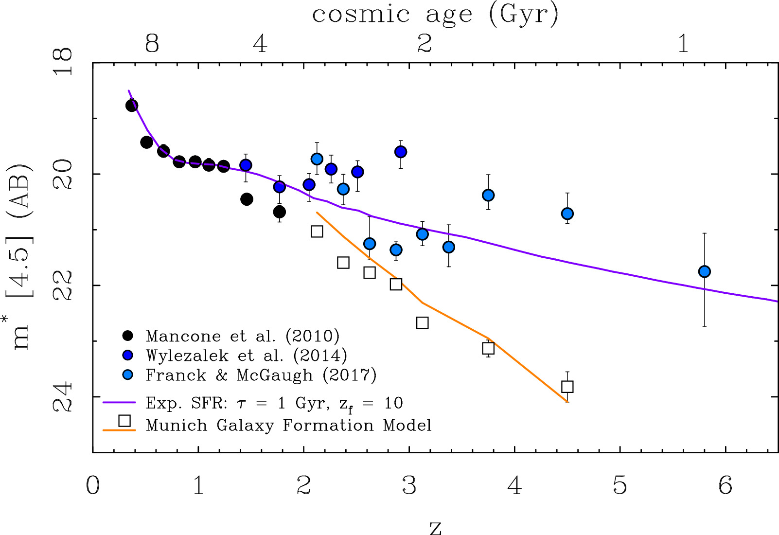
Figure 3. The redshift dependence of the Spitzer [4.5] apparent magnitude m* of Schechter function fits to populations of galaxies in clusters and candidate protoclusters; each point represents all the galaxies in each cluster. Data from C. L. Mancone et al. (2010; black circles), D. Wylezalek et al. (2014; dark blue circles), and J. R. Franck & S. S. McGaugh (2017; blue circles) all have spectroscopic redshifts. The orange line is the prediction of the Munich galaxy formation model (B. M. B. Henriques et al. 2015) based on the Millennium simulations (V. Springel et al. 2005; M. Boylan-Kolchin et al. 2009). Open squares are mock observations of this model using the same algorithm that was applied to the data (J. R. Franck & S. S. McGaugh 2016a). The predicted characteristic magnitude is fainter than observed, diverging systematically for z > 2. The purple line is a model of a galaxy formed at zf = 10 with an exponential star formation history (Equation (1)) with τ = 1 Gyr (J. R. Franck & S. S. McGaugh 2017) normalized at z ≈ 1. Galaxies like this apparently exist in the high-redshift Universe, before they were predicted to have assembled, and are common enough to dominate the Schechter fit for m*.
Download figure:
Standard image High-resolution imageGalaxies become fainter with increasing redshift, as expected (Figure 3). However, observed galaxies are brighter than anticipated by contemporaneous models, e.g., the Munich galaxy formation model (B. M. B. Henriques et al. 2015). The model behaves as expected: earlier galaxies are small protogalaxies, so their characteristic luminosity becomes progressively fainter with increasing redshift. This generic expectation of ΛCDM diverges progressively from the data at z > 2 (Figure 3).
As a check that the same quantity was being measured in both data and model, J. R. Franck (2018) made mock observations of light cones from the Munich model (B. M. B. Henriques et al. 2015). The same algorithm was applied to the mock data that was used to identify protocluster candidates in the real data (J. R. Franck & S. S. McGaugh 2016a, 2016b). The mock observations recover basically the same answer that is known directly from the model (squares in Figure 3). If the real Universe looked like the prediction of the Munich model, we could easily tell. While it is tempting to blame the details of star formation in this particular model, the primary problem is more fundamental. Model galaxies are faint because hierarchical assembly is incomplete at z > 3 (compare Figures 1 and 3).
In contrast, the data fall around the line representing a monolithic giant that formed at zf = 10 and followed an exponential star formation history (Equation (1)). If massive galaxies form early and evolve passively, it would look like the characteristic magnitudes that are observed. In addition to capturing the general trend of the data at high redshift, the data are very well fit at low redshift (z < 1.5). This represents passive stellar evolution over most of cosmic time (∼9 Gyr) after essentially all the stellar mass has been formed and early stochastic variations have had time to subside. These data look very much like the evolution of a massive monolith that was assembled into a single object already at high redshift and not like ΛCDM models in which the largest progenitor should have been much smaller and fainter at z > 2 (Figures 1 and 3).
No single model line will fit all the data in Figure 3. The scatter at high redshift presumably reflects stochastic variations in star formation rates at early times (D. D. Kelson et al. 2016; A. Pallottini & A. Ferrara 2023) before the red sequence was established (E. F. Bell et al. 2004; K. Rakos et al. 2008; J. Schombert & K. Rakos 2009; J. R. Franck et al. 2015). Nevertheless, the evolutionary trend predicted by the monolithic model captures the essence of the data in a way that the nominal prediction of ΛCDM does not.
3.2. Galaxies at z > 6 before JWST
The bulk of the data discussed above are for z < 4 with a couple of candidate protoclusters extending to z ≈ 6 (J. R. Franck & S. S. McGaugh 2016b). There have been many studies of galaxies to yet higher redshift that predate JWST (e.g., A. Grazian et al. 2015; S. L. Finkelstein 2016; M. Song et al. 2016; M. Stefanon et al. 2021; P. Santini et al. 2022; J. R. Weaver et al. 2023). These works provide for field galaxies with stellar mass functions measured independently of any of the data described above, albeit at the cost of relying more, if not entirely, on photometric redshifts.
Figure 4 shows the characteristic stellar mass as a function of redshift. The data from Figure 3 are shown assuming an exponential star formation history to provide a mapping from magnitude to mass that preserves the distribution of the data. This compares well to the data at higher redshift for which the stellar mass estimates are entirely independent (A. Grazian et al. 2015; S. L. Finkelstein 2016; M. Song et al. 2016).
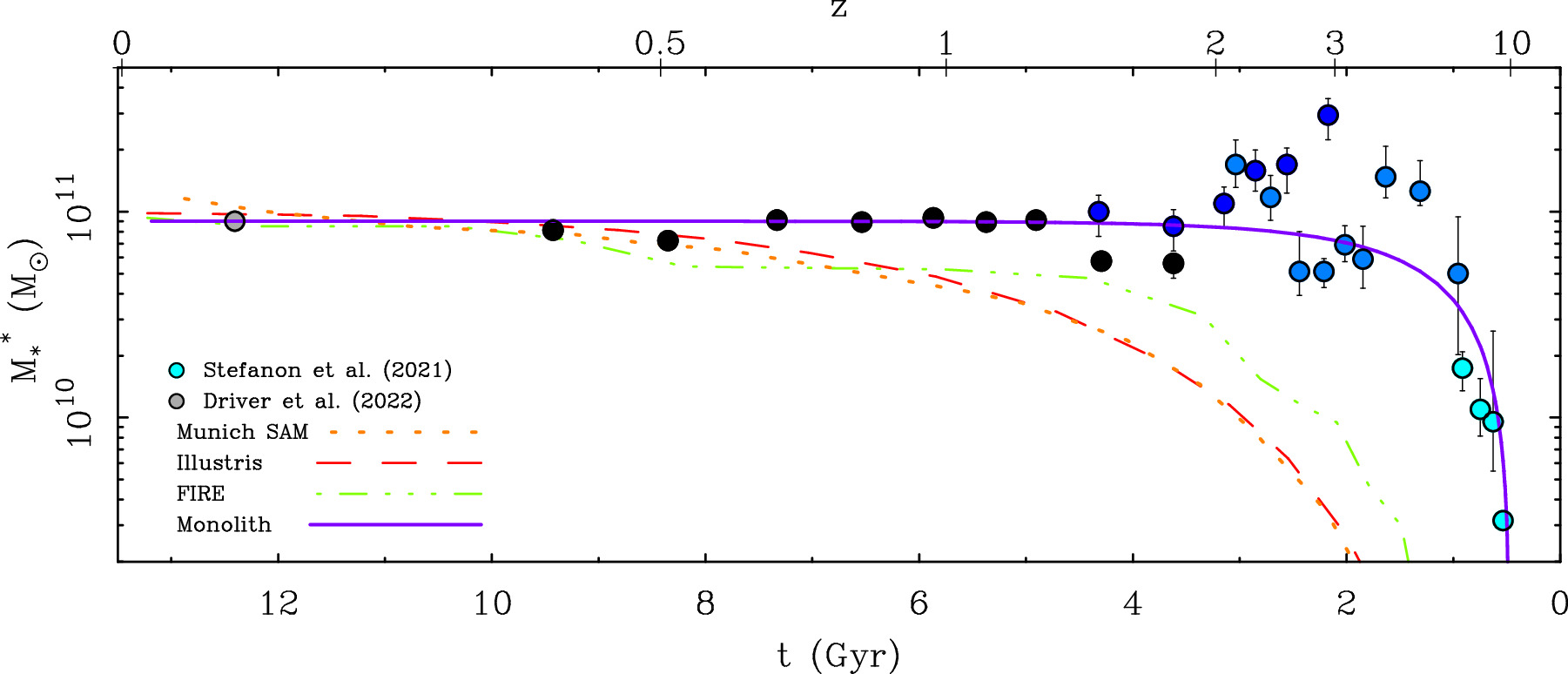
Figure 4. The characteristic stellar mass of the Schechter mass function as a function of time with the corresponding redshift noted at the top. The data from Figure 3 (C. L. Mancone et al. 2010; D. Wylezalek et al. 2014; J. R. Franck & S. S. McGaugh 2017) are augmented with higher-redshift data (M. Stefanon et al. 2021; light blue points). The purple line is the passively evolving monolithic model from Figure 3 normalized to
for local elliptical galaxies (S. P. Driver et al. 2022; gray point). The dotted orange line shows the buildup of the most massive progenitor of a galaxy that reaches this mass by z = 0 in the Munich SAM (B. M. B. Henriques et al. 2015). This is indistinguishable from the result of Illustris (V. Rodriguez-Gomez et al. 2016; red dashed line). Stellar mass in the FIRE simulation (D. Angles-Alcazar et al. 2017; green dotted–dashed line) grows faster, but only a little.
Download figure:
Standard image High-resolution imageWe include in Figure 4 the data of M. Stefanon et al. (2021) together with those from Figure 3. This is the most conservative choice in the sense that the stellar mass estimates of M. Stefanon et al. (2021) are the lowest available at these redshifts. This happens in large part because M. Stefanon et al. (2021) make larger corrections for line emission from nonstellar sources. The data are all consistent; they simply attribute less of the observed luminosity to stars.
The data are consistent with a population of massive galaxies that formed early and evolved passively. Despite its naive simplicity, the exponential star formation history (Equation (3) with τ = 1 Gyr) provides a remarkably reasonable depiction of the buildup of the characteristic stellar mass seen in Figure 4. This is highly nontrivial, as the mass buildup happens early, while the luminosity evolution is most pronounced at late times (Figure 3).
More complex star formation histories are admissible. Indeed, stochastic star formation may well drive the scatter seen in the data around z ≈ 3 when the Universe was only ∼2 Gyr old and stellar populations were necessarily still young. Regardless of the details of the early star formation history, it appears that there exists a population of massive galaxies that formed early and in which most of the stars were made long ago in a single object rather than the multiplicity of progenitors envisioned in hierarchical galaxy formation.
Figure 4 also shows the a priori predictions of several ΛCDM models. These include the Munich SAM (B. M. B. Henriques et al. 2015; as in Figure 3) and the hydrodynamical simulations Illustris (V. Rodriguez-Gomez et al. 2016) and FIRE (D. Angles-Alcazar et al. 2017). These all show basically the same thing. Galaxies are predicted to assemble gradually, with their most massive progenitor not reaching half the final stellar mass until half a Hubble time has passed (z < 1). To give a specific example, the Munich SAM reaches half the final stellar mass at z = 0.68 when the Universe is 7.3 Gyr old. The star formation prescription of FIRE makes more stars earlier, but it is only a small shift of the same basic result: mass assembles too slowly in ΛCDM models. Making star formation more efficient makes more stars earlier, but it does not assemble them into the massive individual galaxies that are observed.
The shortfall of stellar mass in individual galaxies is especially severe at high redshift. At z ≈ 3, the largest progenitor of an L* galaxy is only a tenth of its eventual z = 0 mass in FIRE. It is even less in Illustris, about 3%. At z ≈ 5, individual progenitor galaxies are not expected to have grown massive enough to even appear on Figure 4, let alone to do so at z ≈ 10. Yet at these redshifts, the data show that many galaxies with masses that already approach —enough galaxies to define L* in a Schechter fit for every point in Figure 4. This is the normal galaxy population, not just a few extreme individuals. Moreover, spectroscopic redshifts are required to be a part of the samples (J. R. Franck & S. S. McGaugh 2016a, 2016b) that inform the Schechter function fits of J. R. Franck & S. S. McGaugh (2017), so there is no uncertainty due to photometric redshifts.
JWST has made the observation of galaxies at z > 10 seem mundane, so it is worth recalling that this is a recent development. J. R. Franck & S. S. McGaugh (2017) built the model with zf = 10 shown in Figures 3 and 4 as an extreme upper limit in the context of the widespread presumption at the time that there was no possibility for massive galaxies to have formed that early. Consequently, early JWST results came as a surprise (e.g., E. Merlin et al. 2022; A. Ferrara et al. 2023; S. L. Finkelstein et al. 2023; F. Melia 2023). However, they merely extend the trends already seen in earlier data, corroborating previous indications that galaxies grew too big too fast (B. Rocca-Volmerange et al. 2004; C. L. Steinhardt et al. 2016; J. R. Franck & S. S. McGaugh 2017; E. Merlin et al. 2019). The simple observation is that the high-redshift Universe contains a bounty of bright, morphologically mature galaxies (L. Ferreira et al. 2022, 2023) that are more luminous than had been anticipated by ΛCDM models (e.g., L. Y. A. Yung et al. 2019a, 2022; P. Behroozi et al. 2020).
4.1. The UV Luminosity Function
There is a clear excess in the number density of M* ≈ 1010 M☉ galaxies over the predictions of contemporaneous ΛCDM models (L. Y. A. Yung et al. 2019a, 2019b) at z ≈ 8 (S. S. McGaugh 2024). This becomes more challenging to assess at z > 10, where much of the observed luminosity is in the ultraviolet and the short-lived nature of UV-bright stars makes it difficult to assess the corresponding stellar mass. Bearing this caveat in mind, we can nevertheless compare (Figure 5) observations (C. T. Donnan et al. 2024) with the updated predictions of L. Y. A. Yung et al. (2023). There is a clear excess that is apparent at all luminosities. Similar results follow from comparison to other predictions (e.g., Figure 1; P. Behroozi et al. 2020) and other analyses of the observations (B. Robertson et al. 2024). ΛCDM models did not anticipate the large number of relatively bright galaxies that are observed.
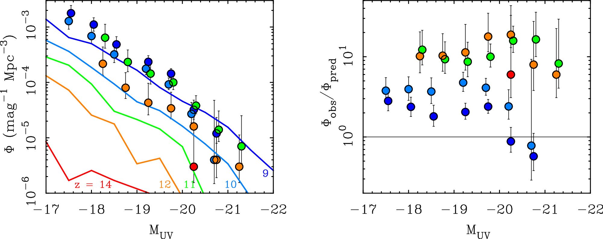
Figure 5. The UV luminosity function (left) observed by C. T. Donnan et al. (2024; points) compared to that predicted for ΛCDM by L. Y. A. Yung et al. (2023; lines) as a function of redshift. Lines and points are color coded by redshift, with dark blue, light blue, green, orange, and red corresponding to z = 9, 10, 11, 12, and 14, respectively. There is a clear excess in the number density of galaxies that becomes more pronounced with redshift, ranging from a factor of ∼2 at z = 9 to an order of magnitude at z ≥ 11 (right).
Download figure:
Standard image High-resolution imageThe excess in the number density of UV-bright galaxies is not subtle, being an order of magnitude at z ≥ 11. This is true despite an upward adjustment of the density in the models by 0.3–0.4 dex from L. Y. A. Yung et al. (2019a) to L. Y. A. Yung et al. (2023). One can imagine a number of ways to further enhance the UV luminosity per unit mass (S. L. Finkelstein et al. 2024), but the salient observational fact is that the UV luminosity function barely evolves over the redshift range over which the dark matter halo mass function is evolving rapidly. Consequently, any appeal to the efficiency of UV light production (or attenuation: A. Ferrara et al. 2023) must necessarily be fine-tuned to balance the barely evolving UV luminosity function with the rapidly evolving dark matter halo mass function over a rather small window of cosmic time, there being only ∼108 yr between z = 14 and 11.
Irrespective of the ultimate interpretation, Figure 5 clearly illustrates the excess in the number of bright high-redshift galaxies over that predicted a priori.
4.2. The Mass and Evolution of Individual Galaxies
Despite the clear excess in bright galaxies seen in Figure 5, it is not yet possible to define a robust population-wide estimate of the corresponding stellar mass as seen in Figure 4. Nevertheless, there are many individual galaxies (Figure 6) that have a reasonably persuasive claim to being high mass at high redshift (S. L. Finkelstein et al. 2022; R. P. Naidu et al. 2022; N. J. Adams et al. 2023; H. Atek et al. 2023; Y. Harikane et al. 2023; I. Labbé et al. 2023; B. Robertson et al. 2024). These are based on photometric redshifts, but similar examples with spectroscopic data are becoming available (B. Wang et al. 2023; S. Carniani et al. 2024; M. Castellano et al. 2024; Y. Harikane et al. 2024; S. H. Price et al. 2024). The essential outstanding feature that they share is how bright they are: galaxies simply do not appear to be as faint as anticipated by ΛCDM models (Figure 3). There are of course some interlopers (P. Arrabal Haro et al. 2023), but changes in the photometric redshift (as sometimes happens; N. J. Adams et al. 2023) do not necessarily reduce the stellar mass, as a reduction in distance is accompanied by a shift of the flux to bands where the stellar mass-to-light ratio is larger than in the UV. The data discussed by I. Labbé et al. (2023) are a case in point: all of the initial redshifts and masses were revised downward after accounting for the on-sky calibration of JWST, but all of them remain problematic in terms of their mass for their redshift.
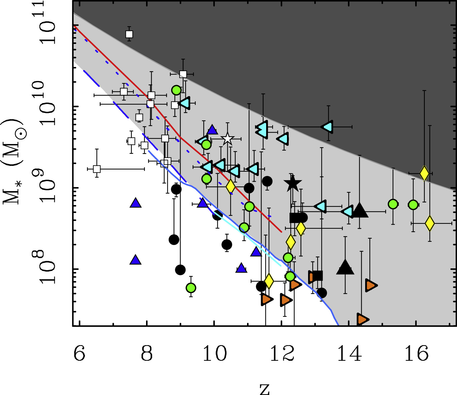
Figure 6. Mass estimates for high-redshift galaxies from JWST. Colored points based on photometric redshifts are from N. J. Adams et al. (2023; dark blue triangles), H. Atek et al. (2023; green circles), I. Labbé et al. (2023; open squares), R. P. Naidu et al. (2022; open star), Y. Harikane et al. (2023; yellow diamonds), C. M. Casey et al. (2024; light blue left-pointing triangles), and B. Robertson et al. (2024; orange right-pointing triangles). Black points from B. Wang et al. (2023; squares), S. Carniani et al. (2024; triangles), Y. Harikane et al. (2024; circles) and M. Castellano et al. (2024; star) have spectroscopic redshifts. The upper limit for the most massive galaxy in TNG100 (V. Springel et al. 2018) as assessed by B. W. Keller et al. (2023) is shown by the light blue line. This is consistent with the maximum stellar mass expected from the stellar mass–halo mass relation of P. Behroozi et al. (2020; solid blue line). These merge smoothly into the trend predicted by L. Y. A. Yung et al. (2019b) for galaxies with a space density of 10−5 dex−1 Mpc−3 (dashed blue line), though L. Y. A. Yung et al. (2023) have revised this upward by ∼0.4 dex (dotted blue line). This closely follows the most massive objects in TNG300 (A. Pillepich et al. 2018; red line). The light gray region represents the parameter space in which galaxies were not expected in ΛCDM. The dark gray area is excluded by the limit on the available baryon mass (P. Behroozi & J. Silk 2018; M. Boylan-Kolchin 2023).
Download figure:
Standard image High-resolution imageFigure 6 shows the stellar masses and redshifts of high-redshift galaxies identified in JWST data. These are individual galaxies rather than the results of Schechter fits to many as in Figure 4. Consequently, they are more plausibly subject to the concern of being rare instances of extreme outliers. To assess the significance of these extreme values, the lines in Figure 6 illustrate the maximum stellar mass found in various studies (L. Y. A. Yung et al. 2019b, 2023; P. Behroozi et al. 2020; B. W. Keller et al. 2023).
To make our own assessment, we queried available simulations to find the most massive model galaxy as a function of redshift. The most generous estimate emerges from the Illustris TNG300 (A. Pillepich et al. 2018) simulation (the red line Figure 6), which closely tracks the estimate of L. Y. A. Yung et al. (2023). These are the most massive objects in a large simulation volume, so observing them would require that JWST happened to observe regions of exceptional overdensity (J. McCaffrey et al. 2023; C. Kragh Jespersen et al. 2024). We therefore consider this line to be a conservative upper limit on stellar mass: objects near this line should be exceedingly rare, and nonexistent beyond it.
There are a number of galaxies observed to exceed the limits illustrated in Figure 6, including cases with spectroscopic redshifts (S. Carniani et al. 2024; Y. Harikane et al. 2024). A few objects approach the limit where all the available baryons would need to already be formed into stars (M. Boylan-Kolchin 2023). These galaxies are difficult to understand in ΛCDM, but they are consistent with a continuation in the trend already seen at intermediate redshift, so they are less surprising from an empirical perspective.
4.3. Quenched Galaxies
Another important observation is that of quenched galaxies at 3 < z < 4 (C. Schreiber et al. 2018; E. Merlin et al. 2019; K. Glazebrook et al. 2024; T. Nanayakkara et al. 2024). These galaxies have observed spectra that show the classic features of a stellar population aging after intense star formation at an earlier epoch. Not only do massive galaxies exist by z ≈ 4, but there are examples that have stellar populations that are old for the age of the Universe at the redshift of observation. By modeling the observed spectra, it is possible to estimate the stellar mass at the time of quenching and roughly when half the stellar mass was in place in addition to the mass at the observed redshift. This provides an approximate curve of growth for each galaxy, as illustrated in Figure 7.
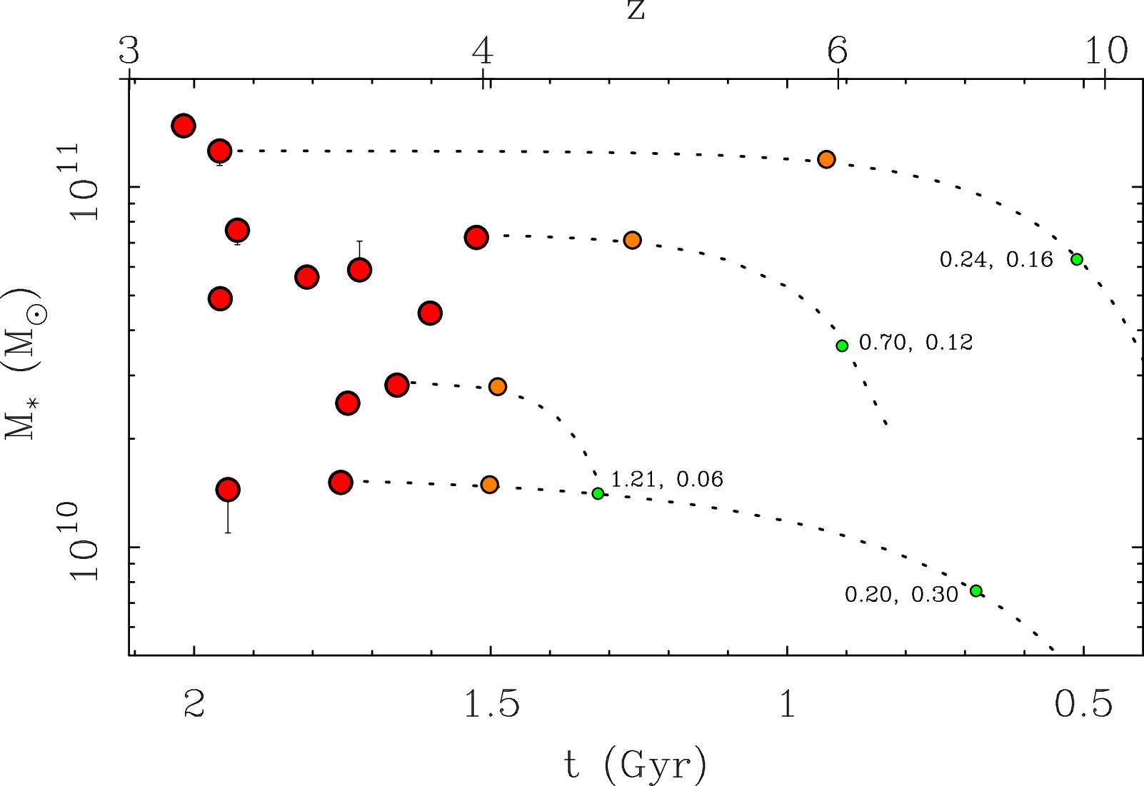
Figure 7. The stellar masses of quiescent galaxies from T. Nanayakkara et al. (2024). The inferred growth of stellar mass is shown for several cases, marking the time when half the stars were present (small green circles) to the quenching time (midsize orange circles) to the epoch of observation (large red circles). Illustrative star formation histories following Equation (5) are shown as dotted lines with parameters ti , τ in Gyr noted. We omit the remaining lines for clarity, as many cross. There is a wide distribution of formation times from very early (ti = 0.2 Gyr) to relatively late (>1 Gyr), but all of the galaxies in this sample are inferred to build their stellar mass rapidly and quench early (τ < 0.5 Gyr).
Download figure:
Standard image High-resolution imageThe growth rates inferred by T. Nanayakkara et al. (2024) are consistent with the rapid rate of growth illustrated by the monolithic model (Equation (5)). Individual galaxies vary in mass, but all are consistent with following a similar evolutionary trajectory. Further examples of such galaxies at yet higher redshift are discussed by B. Wang et al. (2024). These galaxies grew too big too fast, well ahead of the expectation in ΛCDM models.
Galaxies that formed most of their stars early and then quenched are consistent with the traditional view of the evolution of monolithic early-type galaxies. That the galaxies observed by T. Nanayakkara et al. (2024) have masses consistent with other high-redshift galaxies and show the evolved spectra expected for stellar populations descended from earlier star formation suggests that the most obvious interpretation of the data is also the most likely: bright galaxies at high redshift are intrinsically luminous because they contain lots of stars. They appear to have formed as giant monoliths at early times.
The depiction of evolutionary tracks in Figure 7 implicitly assumes that all the mass was assembled at an early time. It is also conceivable that the galaxies observed by T. Nanayakkara et al. (2024) at z ≈ 3–4 were not individual objects at the time of quenching or when half the stellar mass had formed. These events could instead have occurred in protogalactic fragments that subsequently merged to form the observed galaxies. Since the assembled stars are old for the epoch of observation, the assembly must occur as dry mergers devoid of star formation (A. B. Newman et al. 2012; C. J. Conselice et al. 2022).
To check what ΛCDM predicts, we have searched the TNG50 and TNG300 simulations (D. Nelson et al. 2018, 2019) for model galaxies at z = 3 with stellar masses in the same range as the data of T. Nanayakkara et al. (2024). Many examples of such objects exist in the simulations, but almost all are actively star-forming (Figure 8). Quenched galaxies are rare in the simulations at this redshift and nonexistent in the higher-resolution TNG50, with all branches of the merger trees experiencing high specific star formation rates at z > 3 (Figure 1). So while it is possible to find simulated objects of the observed stellar mass, their star formation histories are not a good match to those observed.
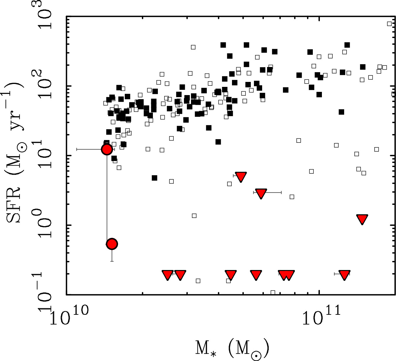
Figure 8. The stellar masses and star formation rates of galaxies from T. Nanayakkara et al. (2024; red symbols). Downward-pointing triangles are upper limits; some of these fall well below the edge of the plot and so are illustrated as the line of points along the bottom. Also shown are objects selected from the TNG50 (A. Pillepich et al. 2019; filled squares) and TNG300 (A. Pillepich et al. 2018; open squares) simulations at z = 3 to cover the same range of stellar mass. Simulated objects with stellar masses comparable to real galaxies are mostly forming stars at a rapid pace. In the higher-resolution TNG50, none have quenched as observed.
Download figure:
Standard image High-resolution imageThe discussion heretofore has focused on the photometric evidence. Kinematic observations provide an independent line of evidence that mature galaxies appeared early in the history of the Universe. Disk galaxies at intermediate redshift (1 < z < 3) are observed to have large rotation speeds (M. Neeleman et al. 2020), be dynamically cold (E. M. Di Teodoro et al. 2016; F. Lelli et al. 2018, 2023; F. Rizzo et al. 2023), and follow scaling relations like Tully–Fisher (S. H. Miller et al. 2012; D. Pelliccia et al. 2017). The Tully–Fisher relation persists up to at least z ≈ 2.5, when the Universe was ∼2.5 Gyr old (A. Nestor Shachar et al. 2023). Individual galaxies with high circular speeds and relatively high rotation-to-velocity dispersion ratios are found up to z ≈ 5 (F. Rizzo et al. 2020, 2021; F. Lelli et al. 2021; F. Roman-Oliveira et al. 2023), barely 1 billion yr after the Big Bang.
The early appearance of massive, dynamically cold disks in the first few billion years after the Big Bang is contradictory to early ΛCDM predictions. For example, H. J. Mo et al. (1998) anticipated that “present-day disks were assembled recently (at z ≤ 1).” Early disks are expected to be small and dynamically hot (A. Dekel & A. Burkert 2014; A. Zolotov et al. 2015; M. R. Krumholz et al. 2018; A. Pillepich et al. 2019). Kinematic scaling relations like Tully–Fisher are expected to emerge late and evolve significantly (e.g., M. Glowacki et al. 2021).
The high rotation speeds observed in early disk galaxies are remarkable. These sometimes exceed 250 (M. Neeleman et al. 2020) or even 300 km s−1(A. Nestor Shachar et al. 2023; W. Wang et al. 2024), comparable to the most massive local spirals (E. Noordermeer et al. 2007; E. M. Di Teodoro et al. 2021, 2023). Kinematics indicate large dynamical masses for these early galaxies. The problem is not limited to luminosity; the underlying dynamical mass is also larger than expected.
The study of kinematics at still higher redshift is a nascent field, but there are already important individual cases. For example, the kinematics of ALESS 073.1 at z ≈ 5 indicate the presence of a massive stellar bulge as well as a rapidly rotating disk (F. Lelli et al. 2021). A similar case has been observed at z ≈ 6 (R. Tripodi et al. 2023). These kinematic observations indicate the presence of mature, massive disk galaxies well before they were expected to be in place (A. Pillepich et al. 2019; J. Wardlow 2021). Spiral galaxies are ubiquitous in JWST images up to z ∼ 6 (L. Ferreira et al. 2022, 2023; V. Kuhn et al. 2024).
Figure 9 shows two scaling relations at both low and high redshift: the baryonic mass–circular speed relation (R. B. Tully & J. R. Fisher 1977; S. S. McGaugh et al. 2000) and the dark matter fraction–surface brightness relation (W. J. G. de Blok & S. S. McGaugh 1997; N. Starkman et al. 2018). Both relations are clearly present in the data of A. Nestor Shachar et al. (2023). There is little if any indication of evolution in either relation up to z ≈ 2.5. The good agreement between low- and high-redshift samples is remarkable given that we have made no attempt to reconcile the choice of circular velocity measure (F. Lelli et al. 2019) or the precise definition of baryonic mass, which is sensitive to the stellar population model and its evolution (J. Schombert et al. 2019). Any systematic differences between studies are apparently within the scatter induced by measurement uncertainties.
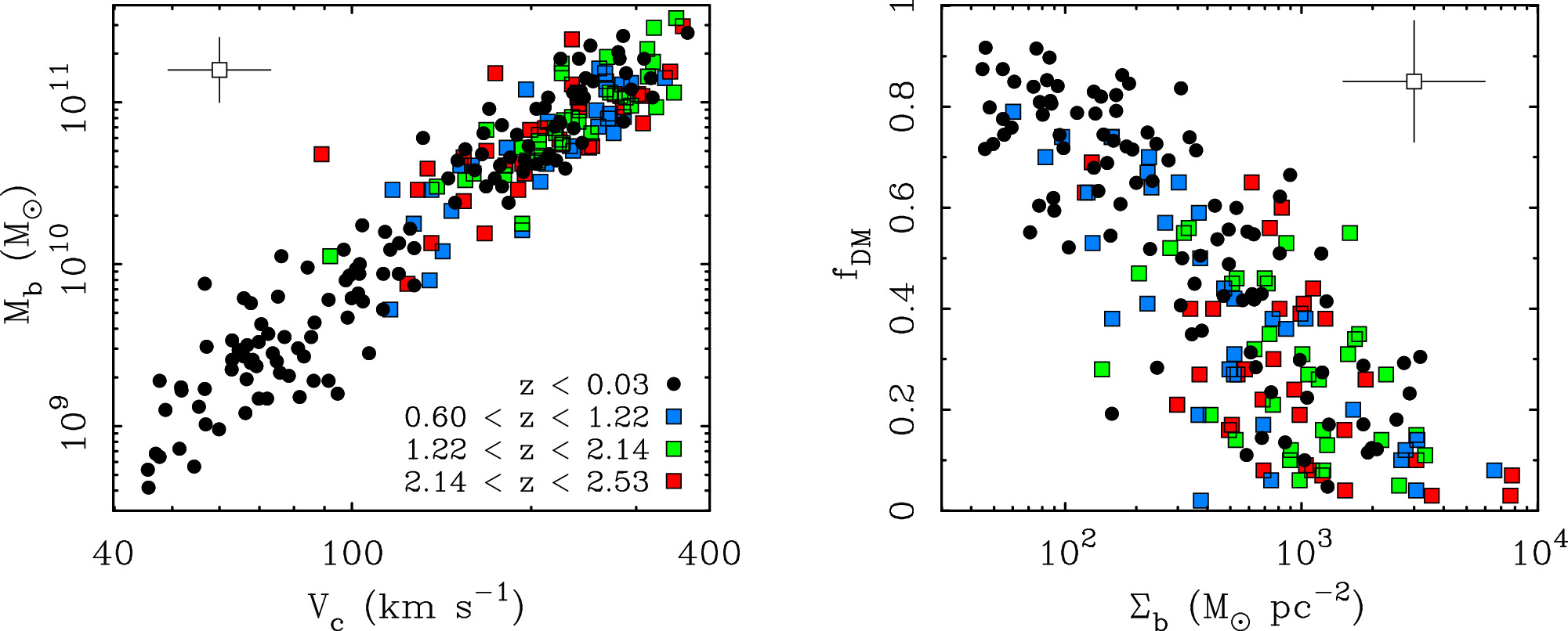
Figure 9. The baryonic Tully–Fisher (left) and dark matter fraction–surface brightness (right) relations. Local galaxy data (circles) are from F. Lelli et al. (2019; left) and F. Lelli et al. (2016; right). Higher-redshift data (squares) are from A. Nestor Shachar et al. (2023) in bins with equal numbers of galaxies color coded by redshift: 0.6 < z < 1.22 (blue), 1.22 < z < 2.14 (green), and 2.14 < z < 2.53 (red). Open squares with error bars illustrate the typical uncertainties. The relations known at low redshift also appear at higher redshift with no clear indication of evolution over a lookback time up to 11 Gyr.
Download figure:
Standard image High-resolution imageThe dark matter fraction , where Vc
is the observed circular velocity and Vb
is that due to the baryons at the same radius. Many high surface brightness galaxies are maximal in their inner regions, so Vb
→ Vc
and fDM → 0 (N. Starkman et al. 2018). The precise value of fDM is very sensitive to the stellar population model, which determines the amplitude of Vb
. This is less critical for low surface brightness galaxies, which have long been known to be dark-matter-dominated (W. J. G. de Blok & S. S. McGaugh 1997). Figure 9 shows that the relation between the dark matter fraction and surface brightness was already in place at intermediate redshift (A. Nestor Shachar et al. 2023) and has not evolved much over cosmic time (G. Sharma et al. 2023).
Kinematic observations to date show that dynamically cold, massive disks are already present in the Universe at early times. These disk galaxies appear to follow the same kinematic scaling relations that are known locally. The presence of dynamically massive galaxies in settled kinematic scaling relations at early times does not follow naturally from the hierarchical galaxy formation picture.
ΛCDM galaxy formation models (e.g., B. M. B. Henriques et al. 2015; V. Rodriguez-Gomez et al. 2016; D. Angles-Alcazar et al. 2017; L. Y. A. Yung et al. 2019b; P. Behroozi et al. 2020) failed to anticipate the bright galaxies that are observed at both intermediate and high redshift. Forming enough stars is not the problem. The problem is assembling them into a single object. The presence of these quasi-monolithic objects appears to violate the hierarchical assembly paradigm.
6.1. Observed Numbers and the Mass Function
There are two basic issues, one theoretical and one observational. On the theory side, we must be careful about what the theory predicts, including the inherent uncertainties in doing so. The mass function of the dark matter halos is well predicted, but relating this to stellar mass requires a prescription for the star formation efficiency. Relating the mass of stars formed to the observed magnitudes requires a stellar population model. These are good, but never perfect. Stellar population models also play a role on the observational side in fitting the observed spectral energy distribution to obtain a simultaneous estimate of the stellar mass and redshift. This process can go amiss (e.g., N. J. Adams et al. 2024), but enough spectroscopic observations now exist (B. Wang et al. 2023; S. Carniani et al. 2024; M. Castellano et al. 2024; Y. Harikane et al. 2024; S. H. Price et al. 2024) that it seems unlikely that the whole problem can be one of misleading observations.
The normalization of numerical simulations is not trivial. L. Y. A. Yung et al. (2023) reassessed their predictions (L. Y. A. Yung et al. 2019b) in the light of higher-resolution simulations. This resulted in an upward shift in numbers at a given redshift by a factor of ∼2 (Figure 6). This helps, but only a bit. There remain galaxies of larger mass at higher redshift than should be possible, including examples with spectroscopic redshifts (B. Wang et al. 2023; S. Carniani et al. 2024).
In contrast, H. Katz et al. (2023) find a good match of the Sphinx simulation (J. Rosdahl et al. 2018, 2022) with the cumulative number counts at 9 < z < 13. In this case, the test may come at lower redshift, to which it is not yet computationally feasibly to extend Sphinx. Figure 34 of H. Katz et al. (2023) shows the surface density n(z) increasing rapidly with decreasing redshift, implying that this simulation may fit the high-redshift data at the risk of overshooting the data at lower redshift (E. Merlin et al. 2019; N. Sabti et al. 2024). The evolutionary trajectories that are common in simulations do not have the right shape to explain the data (Figure 10).
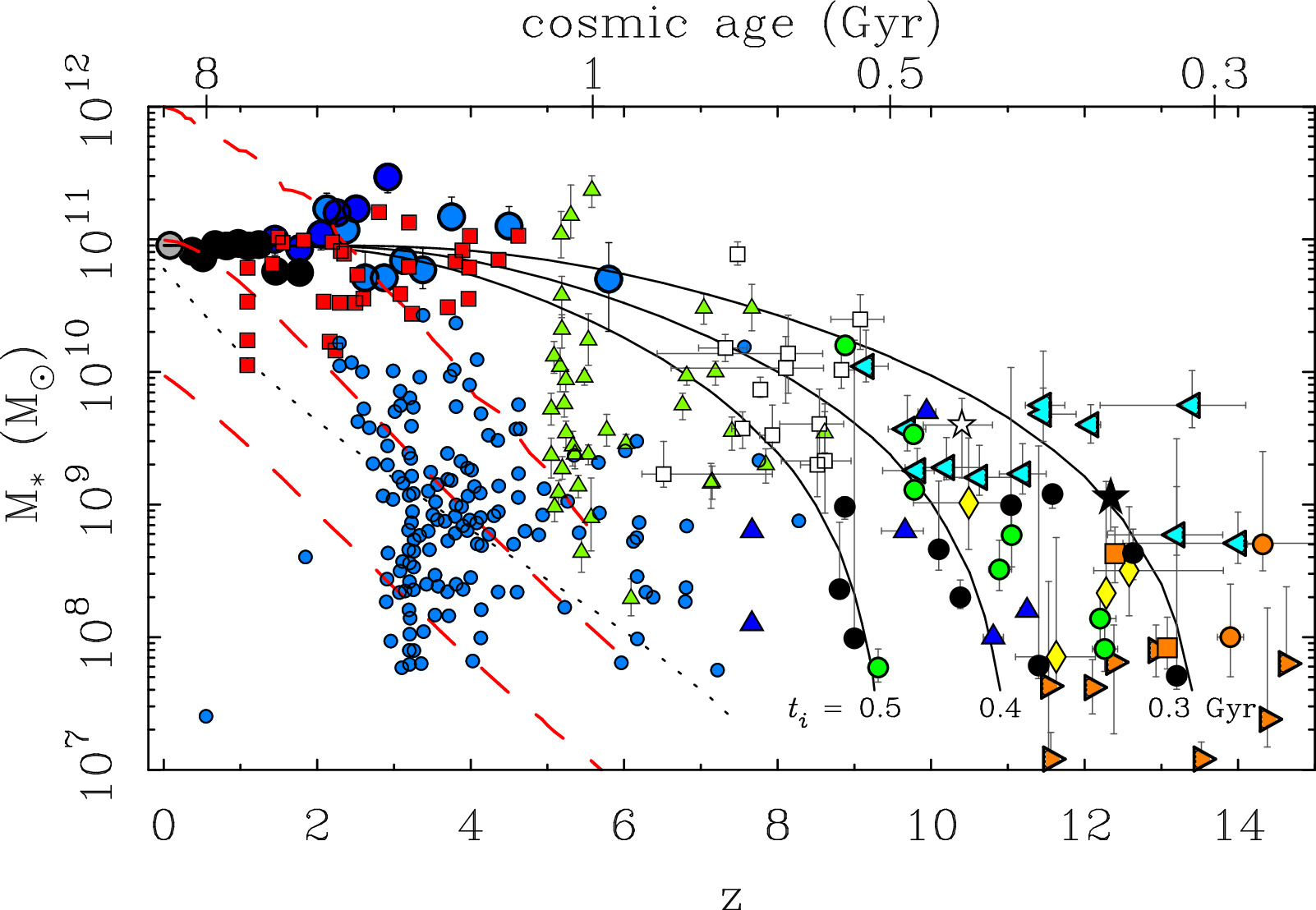
Figure 10. The data from Figures 4 and 6 shown together using the same symbols. Additional JWST data with spectroscopic redshifts are shown from M. Xiao et al. (2023; green triangles) and A. C. Carnall et al. (2024). The data of A. C. Carnall et al. (2024) distinguish between star-forming galaxies (small blue circles) and quiescent galaxies (red squares); the latter are in good agreement with the typical determined from Schechter fits in clusters (large circles). The dashed red lines show the median growth predicted by the Illustris ΛCDM simulation (V. Rodriguez-Gomez et al. 2016) for model galaxies that reach final stellar masses of M* = 1010, 1011, and 1012
M☉. The solid lines show monolithic models with
and ti
= τ = 0.3, 0.4, and 0.5 Gyr (Equation (5)), as might be appropriate for giant elliptical galaxies. The dotted line shows a model appropriate to a spiral galaxy with ti
= 0.5 and τ = 13.5 Gyr.
Download figure:
Standard image High-resolution image6.2. Evolutionary Trajectories
The expectation of hierarchical galaxy formation in ΛCDM is illustrated in Figure 1. The stellar mass of a galaxy is a combination of in situ star formation in its largest progenitor and ex situ star formation in a multitude of protogalactic clumps that ultimately merge into it. This is a gradual process, with the median stellar mass reaching half its final value at z < 1 (G. De Lucia et al. 2006; G. De Lucia & J. Blaizot 2007; V. Rodriguez-Gomez et al. 2016; D. Angles-Alcazar et al. 2017). The brightness of the typical galaxy is thus expected to diminish rapidly as we look to high redshift (Figure 3), both because the largest progenitor is smaller and less mature and because it should split into many precursor protogalaxies. Here the simple monolithic galaxy model provides a useful contrast in which all the baryons assemble promptly at an early time and the luminosity evolution is due entirely to in situ star formation.
Figure 10 combines the data from Figures 4 and 6 to show the stellar mass of galaxies observed over all of accessible cosmic time. These data are further augmented with recent spectroscopic observations by M. Xiao et al. (2023) and A. C. Carnall et al. (2024). The data begin to fill out the stellar mass–redshift diagram, with only the top right portion of Figure 10 being empty. The remainder of the diagram is populated by galaxies of a wide range of masses and evolutionary states.
The hierarchical ΛCDM model is represented in Figure 10 by three evolutionary tracks from the Illustris simulation (M. Vogelsberger et al. 2014). These illustrate the median stellar mass growth of the largest progenitors that reach , 1011, and 1012
M☉ at z = 0 (V. Rodriguez-Gomez et al. 2016). These trajectories parallel one another, with the primary difference being that in normalization. These are typical objects; atypical objects also follow a similar trajectory with a higher or lower normalization (e.g., the maximum stellar mass line in Figure 6). Other ΛCDM simulations (e.g., D. Angles-Alcazar et al. 2017; H. Katz et al. 2023) follow similar trajectories with modest variations (Figure 4). These variations stem from differences in the implementation of baryonic physics, not in the more fundamental assembly of mass.
Monolithic models that form early and reach a mass of at z = 0 are shown with three lines that follow Equation (5) with ti
= τ = 0.3, 0.4, and 0.5 Gyr. These represent the traditional picture of a giant elliptical galaxy that is in place early, forms its stars in an initial burst, and evolves passively thereafter. A giant spiral model is also illustrated with ti
= 0.5 and τ = 13.5 Gyr to show the effect of a more extended period of star formation.
The evolutionary tracks of the monolithic models naturally explain the high-redshift (z > 6) region of the M*–z plane. This region is not explored by the ΛCDM tracks and is not accessible to typical ΛCDM models; we must appeal to rare outliers. The reason for this not merely a difference in star formation history; it is a consequence of the time required to hierarchically assemble mass (Figure 1). Observed galaxies appear to have assembled more promptly than anticipated by ΛCDM. A deviation from the predicted hierarchical assembly of mass is a considerably greater problem for ΛCDM than the details of star formation in the largest progenitor.
Another problem is the shape of the simulated ΛCDM evolutionary tracks. The tracks are nearly linear in Figure 10. This is fine for assembling a spiral galaxy with an extended star formation history, but it is the wrong shape to describe the upper envelope of the data. If a rare outlier is invoked to explain massive galaxies at high redshift, the growth tracks predict that the low-redshift descendant of this object will be more massive than anything in the local Universe.
In contrast, the shape of the monolithic model is a good match to the distribution of the data. It traces the envelope of the most massive galaxies at high redshift and arrives at a plausible mass at low redshift. The monolithic model is also consistent with quenched galaxies being common at intermediate redshifts. Objects that form quickly with short star-forming timescales (τ ≲ 1 Gyr) form the bulk of their stars early (Figure 4) and so should appear quenched.
It appears to us that the problem is the mass assembly history, not the star formation history. If correct, this implies that the hierarchical galaxy formation paradigm is broken; this would be a fundamental challenge to ΛCDM. However, we have considerable freedom to adjust the star formation history of protogalaxies at early times, so we consider this and other possibilities below.
6.3. Possible Solutions
It is conceivable that we have the cosmology wrong (P. Li 2023; F. Melia 2023). Short of that, there are a number of auxiliary hypotheses that we might invoke to attempt to save the phenomena. In a nutshell, we need to find a way to make the evolution of the brightest progenitor look like a monolithic model (Figure 1).
There is a strong selection effect to see the brightest objects at the limit of our observations, so perhaps the bright galaxies observed at high redshift are rare outliers (e.g., J. McCaffrey et al. 2023; C. Kragh Jespersen et al. 2024). This idea is challenged by the number of objects that exceed the extremal estimates for the single most massive object that can appear as a function of redshift (Figure 6). It suffers even greater problems explaining the data at intermediate redshift (z ≈ 3–4), where mature, massive (M* ≈ 1011 M☉) galaxies exist (C. Schreiber et al. 2018; E. Merlin et al. 2019; K. Glazebrook et al. 2024; T. Nanayakkara et al. 2024). These objects were not anticipated to exist in ΛCDM and cannot be attributed to rare outliers, as they are common enough to define L* in Schechter fits (D. Wylezalek et al. 2014; C. L. Steinhardt et al. 2016; J. R. Franck & S. S. McGaugh 2017). Rare objects may be part of the solution, but rarity by itself does not suffice.
At the highest redshifts, much of the observed light is from the rest-frame ultraviolet, which is subject to the considerable uncertainty associated with massive stars and their short lifetimes (S. L. Finkelstein et al. 2024). An obvious possibility is a top-heavy initial mass function (T. Harvey et al. 2024) that enhances the production of UV light per unit mass. This seems unlikely to maintain the nearly constant UV luminosity function that is observed as the underlying halo mass function evolves rapidly with redshift (Section 4.1). This possibility is difficult to test, but it also does not sit well with the observation of quenched galaxies at intermediate redshift that appear to be the descendants of normal stellar populations.
Some of the bright sources could be active galactic nuclei (AGN) instead of galaxies. This possibility seems unlikely now that spectroscopic observations plainly reveal the spectra of normal stellar populations (M. Xiao et al. 2023; A. C. Carnall et al. 2024; S. H. Price et al. 2024). That excessively bright sources might be AGN was considered by J. R. Franck & S. S. McGaugh (2017), who found that the inference of numerous bright galaxies persisted even if the brightest sources were ignored. Invoking AGN does not really help anyway, as it simply turns the problem of too many early stars into one of too many early supermassive black holes.
Perhaps the most obvious possibility is that star formation is more efficient at high redshift so that more of the available baryons form into stars (e.g., M. Xiao et al. 2023; A. C. Carnall et al. 2024; J.-C. Wang et al. 2024). This line of reasoning has a limit, as star formation cannot be more efficient than 100%: there comes a point when dark matter halos lack enough baryons to produce the observed stars (M. Boylan-Kolchin 2023). A few galaxies appear to challenge this disallowed region (Figure 6), albeit not many. While these may prove illusory (P. Arrabal Haro et al. 2023), there do seem to be a number of high-redshift galaxies for which the stellar fraction approaches the limit of the available baryons (f* → 1; M. Xiao et al. 2023; A. C. Carnall et al. 2024). This is apparently necessary to maintain consistency with ΛCDM (A. C. Carnall et al. 2024; J.-C. Wang et al. 2024).
One does not simply turn all the available baryons into stars. Local star formation is nowhere near that efficient (A. K. Leroy et al. 2008), and we find it difficult to imagine that it can be. The net result must be to form enough stars early on to mimic a monolithic model as seen in Figure 10. This is a big ask, as the star formation must not only be highly efficient, it must then rapidly quench (L. C. Kimmig et al. 2023). Such models must also respect the limit on the baryon content of galaxies, which is typically low (f* < 0.5) at low redshift (S. S. McGaugh et al. 2010).
Some sort of superefficient star formation (SESF) appears necessary at early times to maintain consistency with ΛCDM. This is a mode of star formation that is utterly unfamiliar in the local Universe. We briefly speculate on the conditions in the early Universe that may lead to SESF. First, it seems likely that SESF, if it happens, contributes to the formation of giant elliptical galaxies. These may be associated with somewhat rare peaks in the initial power spectrum that preferentially reside in dense environments. Since structure correlates with structure, we imagine that these protogalaxies have a large amount of substructure. In effect, the bottom tier of the merger tree in Figure 1 starts in a dense configuration. We then imagine that there is some threshold for SESF that is crossed once a sufficient density of substructure is obtained, and the evolution proceeds rapidly in a manner reminiscent of violent relaxation (D. Lynden-Bell 1967).
This crude outline is not guaranteed to happen, much less to drive star formation so efficient that f* → 1. To achieve something like SESF, the mode of star formation needs to change dramatically once an arbitrary threshold distinguishing protoellipticals from protospirals is crossed. For this to work, it is necessary for feedback to be suppressed so that star formation can completely consume the available baryons. This seems outlandish but is perhaps the least outlandish of the available options.
It is necessary to invoke auxiliary hypotheses like SESF to avoid the conclusion that observations of the high-redshift Universe are genuinely problematic for ΛCDM (M. Haslbauer et al. 2022b). Indeed, the usual linear growth rate cannot reconcile the new JWST results with previous results from HST (N. Sabti et al. 2024) without invoking such extreme hypotheses. Perhaps the data themselves indicate nonlinearity.
That structure could and should form at an accelerated pace was anticipated well in advance by R. H. Sanders (1998, 2008), S. Stachniewicz & M. Kutschera (2001), S. S. McGaugh (2004, 2018), C. Llinares et al. (2008), and others; see S. S. McGaugh (2015) and references therein. The new physics driving the prediction of early structure formation is MOND (M. Milgrom 1983). MOND has a lengthy track record of predictive success (M. Milgrom 2014), many aspects of which are not satisfactorily explained by dark matter (S. McGaugh 2020). The early formation of massive galaxies is another predictive success.
R. H. Sanders (1998) was the first to explicitly predict that “Objects of galaxy mass are the first virialized objects to form (by z = 10).” Contrast this with the contemporaneous ΛCDM statement by H. J. Mo et al. (1998): “present-day disks were assembled recently (at z ≤ 1).” One of these a priori predictions is consistent with the data.
The work of R. H. Sanders (2008) anticipates the success of the monolithic model seen above. The observation of bright, massive galaxies at high redshift is precisely what is expected in MOND (Figure 2). The assembly of mass is greatly accelerated by the nonlinearity of MOND (A. Nusser 2002); there is no need to invoke SESF or other unlikely effects.
To a good approximation, galaxies in MOND evolve as monolithic island Universes after a chaotic early period of hierarchical assembly. This hierarchical assembly is greatly accelerated by the nonlinearity of MOND relative to the linear case of ΛCDM. In situ growth dominates, and galaxies follow an evolutionary path dictated by the usual astrophysics of gas accretion, cooling, star formation, and feedback (F. Combes 2014). Mergers certainly continue to happen at late times but over longer timescales and with less frequency than in ΛCDM (O. Tiret & F. Combes 2008).
Observations at z ≳ 15 may reveal the rapid early assembly of the first giant galaxies. The transition from hierarchical to monolithic behavior should be sudden and likely lies in the range 15 < z < 20. However, the precise timing is highly dependent on the underlying cosmology, which need not follow ΛCDM exactly at these redshifts, where there are few empirical constraints on the expansion history of the Universe and the corresponding time–redshift relation (S. S. McGaugh 2018). This depends on the underlying theory, which may be a generalization of general relativity along the lines discussed by C. Skordis & T. Złosnik (2019). Exactly what this theory is remains a profound question.
7.1. Clusters
A further prediction of R. H. Sanders (1998) is that “larger structure develops rapidly.” For example, massive clusters of galaxies should form early in MOND. A region destined to become a cluster of galaxies will reach maximum expansion after 2–3 Gyr (Figure 2), so clusters should emerge as recognizable objects fairly early in the development of the Universe.
The predicted emergence of clusters in MOND is certainly earlier than anticipated in ΛCDM. A. V. Kravtsov & S. Borgani (2012) show that a ∼1015 M☉ cluster is barely getting started at z = 3 (see their Figure 6). Note that in MOND, there is no cold dark matter, so the equivalently massive cluster is of order 1014 M☉. R. H. Sanders (1998) predicts “that by z = 3 not only do massive galaxies exist but they are also significantly clustered (the density of the 1014 M☉ region would be enhanced by a factor of 6.5 over the mean at this redshift).”
J. R. Franck & S. S. McGaugh (2016a, 2016b) identify dozens of protocluster candidates at redshifts 2 < z < 6.6 (Figure 11). Of these, the 16 most reliable candidates have N ≥ 10 spectroscopically confirmed members with overdensities ranging from 5 to 20 with a median δ = 9.5. Similar structures have recently been identified by N. Laporte et al. (2022), who identify a protocluster candidate at z = 7.66; T. Morishita et al. (2023), who find another protocluster at z = 7.88; and E. A. Shah et al. (2024), who identify six massive protoclusters around z ≈ 3. This is consistent with the findings of J. R. Franck & S. S. McGaugh (2016b) and the predictions of MOND. Clusters should not appear this early in ΛCDM (M. J. Mortonson et al. 2011; A. V. Kravtsov & S. Borgani 2012).
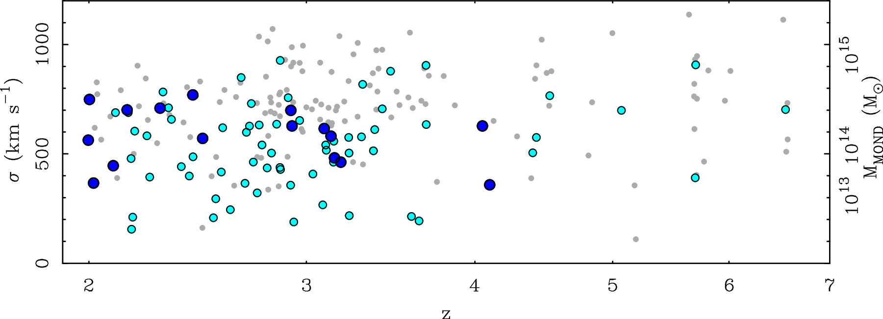
Figure 11. Measured velocity dispersions of protocluster candidates (J. R. Franck & S. S. McGaugh 2016a, 2016b) as a function of redshift. Point size grows with the assessed probability that the identified overdensities correspond to a real structure: all objects are shown as small points, candidates with P > 50% are shown as light blue midsize points, and the large dark blue points meet this criterion and additionally have at least 10 spectroscopically confirmed members. The MOND mass for an equilibrium system in the low-acceleration regime is noted at right; these are comparable to cluster masses at low redshift.
Download figure:
Standard image High-resolution imageA number of the best candidate clusters of J. R. Franck & S. S. McGaugh (2016a, 2016b) are at z ∼ 3. The median velocity dispersion of candidate clusters is ∼600 km s−1 (Figure 11). This is about twice that of equivalent systems found in lookback cones in ΛCDM simulations (J. R. Franck 2018). That is, protocluster candidates identified as spikes in N(z) have larger velocity dispersions in the data than in simulations at the same redshift. This is another indication that the discrepancy is one in mass, not just luminosity. These systems should not yet be bound in ΛCDM, but it is possible that they have already formed in MOND (Figure 2).
The median observed velocity dispersion of intermediate-redshift cluster candidates corresponds to a mass of ∼1014 M☉ for systems in dynamical equilibrium in the deep MOND regime of low acceleration (≪a0). These numbers are very much in line with the long-standing prediction of R. H. Sanders (1998) and are similar to the masses inferred for clusters in MOND at low redshift (S. S. McGaugh 2015; P. Li et al. 2023; Y. Tian et al. 2024). Galaxy clusters are known to display a residual mass discrepancy in MOND of about a factor of 2 (R. H. Sanders 2003, 2007; G. W. Angus et al. 2008), so there is an apparent need for an extra mass component, possibly in the form of undetected baryons (M. Milgrom 2008; R. Kelleher & F. Lelli 2024). We are thus in the curious situation that the masses of galaxy clusters are problematic for MOND, but their formation time is potentially problematic for ΛCDM, as are other properties like cluster collision speeds (G. W. Angus & S. S. McGaugh 2008; H. Katz et al. 2013) and the largest-mass objects (E. Asencio et al. 2021).
7.2. Larger Structures
The morphology of cosmic structure is similar in ΛCDM and MOND (C. Llinares et al. 2008; S. S. McGaugh 2015), but the accelerated structure formation of MOND pushes all benchmarks for structure formation to earlier times in cosmic history. This provides a natural explanation for the strong clustering of high-redshift quasars (e.g., Y. Shen et al. 2007; R. G. Clowes et al. 2013; J. D. Timlin et al. 2018; A.-C. Eilers et al. 2024; E. Pizzati et al. 2024) and other very large features (I. Horváth et al. 2014, 2015; L. G. Balázs et al. 2015; A. M. Lopez et al. 2022; E. Ó. Colgáin et al. 2024). These features are larger than expected in ΛCDM but quite natural in MOND.
Another indication of early structure is that clusters already appear themselves to be clustered at high redshift (J. R. Franck & S. S. McGaugh 2016b). This is visible in Figure 11 as the multiplicity of objects at similar redshift, e.g., at z ≈ 5.7 and z ≈ 6.6. In addition to explaining unexpectedly overdense regions, MOND is also effective at making large, empty voids (C. Llinares et al. 2008; S. S. McGaugh 2015), a persistent puzzle in ΛCDM (A. Nusser et al. 2005; P. J. E. Peebles & A. Nusser 2010).
R. H. Sanders (1998) notes that the largest structures nearing turnaround today would be superclusters (S. Sankhyayan et al. 2023). These are not expected to be simple objects, as they are inevitably far from the simple spherical approximation of Equation (6). Indeed, it was recognized early (J. E. Felten 1984) that MOND would induce anisotropy on unexpectedly large scales. These considerations anticipate the size and complex kinematics of objects like Laniakea (R. B. Tully et al. 2014) and Ho’oleilana (R. B. Tully et al. 2023).
At late times, it becomes difficult for the entire Universe to remain isotropic (J. E. Felten 1984) in MOND. This motivates searches for anisotropy in the expansion rate (J. Colin et al. 2019; W. Rahman et al. 2022; P. Kumar Aluri et al. 2023; C. A. P. Bengaly et al. 2024) and would go some way to explain the tension between the dipole anisotropy of number counts of distant sources and the cosmic microwave background (N. J. Secrest et al. 2021, 2022; G. Domènech et al. 2022).
7.3. Early Reionization
S. S. McGaugh (2004) predicted that “the most obvious signature of MOND-induced structure formation is an early onset of reionization.” This is a natural consequence of early structure formation. The reionization of the Universe is achieved by the ultraviolet radiation of conventional sources like Population II stars. It will be patchy and require an extended time to complete, starting around z ≈ 17 (S. S. McGaugh 2004, 2018). The uncertainty in the precise redshift of onset is large thanks to the inverse relation between time and redshift. The onset of patchy reionization earlier than z ≳ 12 favors MOND over ΛCDM.
JWST observations are beginning to show signs of the predicted early reionization. M. Tang et al. (2024) find indications of patchy reionization, with some lines of sight being transparent to Lyα photons to surprisingly high redshift (z ∼ 8). These are the bubbles of early reionization, as expected in MOND.
There is also an apparent crisis in the budget of UV photons at high redshift (J. B. Muñoz et al. 2024). JWST observations are in tension with the optical depth due to Thomson scattering estimated in fits to Planck data (τ = 0.058 ± 0.006; M. Tristram et al. 2024). This quantity is covariant with other parameters in such fits; a higher optical depth τ ≈ 0.17 provides a good fit to the Planck data at ℓ < 600 in the absence of cold dark matter (S. S. McGaugh 2004). The high density of UV photons observed by JWST is as expected in MOND. A further consequence of early reionization is an enhanced Integrated Sachs-Wolfe (ISW) effect (S. S. McGaugh 2004), for which there is some evidence (B. R. Granett et al. 2008; S. Nadathur et al. 2012; A. Kovács et al. 2020).
The early onset of structure formation has further consequences for the high-redshift Universe. Predictions for 21 cm absorption at cosmic dawn and during the dark ages are discussed by S. S. McGaugh (2018). The depth of the absorption signal can be deeper than in ΛCDM at both epochs (z ≈ 17 and z ≈ 100). The redshift-dependent power spectrum contains further clues. Due to the nonlinear growth of structure, one expects little power in fluctuations entering the dark ages (z ∼ 150) but more by their end (z ∼ 50) in MOND than in ΛCDM. These would be clear signs of nonlinear structure formation and a departure from the ΛCDM cosmology.
We have examined evidence concerning the evolution of galaxies across a large range of redshifts for which data are available. There appears to be a population of bright galaxies that formed early and grew rapidly. There is copious photometric evidence that indicates the existence of this population and important corroborative evidence from kinematics.
8.1. Photometric Evidence
The galaxy population that grew too big too fast has photometric properties that suggest it is
1.
luminous, with apparent magnitudes considerably brighter than anticipated by contemporaneous ΛCDM models (Figure 3);
2.
massive, with typical examples approaching the mass of a local L* galaxy already by z ≈ 3, when the Universe was only ∼2 Gyr old (Figure 4);
3.
old, with stellar populations consistent with forming at high redshift, zf ≳ 10 (Figures 7 and 10), and quenching early (Figure 8);
4.
common in clusters at z ≲ 3 and already clustered in protoclusters at z ≲ 6 (Figure 11); and
5.
consistent with the population of bright galaxies observed by JWST at z > 10 (Figure 10), where bright galaxies are more common than anticipated (Figures 5 and 6).
These observed properties do not sit well with hierarchical ΛCDM models, which predict that local massive galaxies were divided into many progenitor protogalaxies at the observed redshifts (Figure 1). A more natural interpretation is that galaxies are bright at high redshift because they had already grown large. This provides an evolutionary trajectory that maps nicely between observations at low, intermediate, and high redshift. Note that it is not necessary for all galaxies to form early and follow such a trajectory, just enough of them to define a bright L* in early (z ≈ 3) clusters (J. R. Franck & S. S. McGaugh 2017). This population was not anticipated by ΛCDM models and is not easily reconciled with them; these galaxies grew too big too fast.
8.2. Kinematic Evidence
Photometric observations are complemented by kinematic observations that trace the mass, not just the light. JWST observations show that morphologically mature spiral galaxies are common at early times (L. Ferreira et al. 2022, 2023). Kinematic observations to date (Section 5) show that rotationally supported galaxies
1.
formed early, by z ≳ 6 (R. Smit et al. 2018; L. E. Rowland et al. 2024; Y. Xu et al. 2024), when z ≤ 1 had been the nominal expectation (H. J. Mo et al. 1998);
2.
rotate fast, with circular speeds in excess of 250 km s−1 (F. Lelli et al. 2021; F. Rizzo et al. 2021), comparable to massive local spirals;
3.
obey the baryonic Tully–Fisher relation (F. Lelli et al. 2018, 2019; A. Nestor Shachar et al. 2023); and
4.
obey the dark matter fraction–surface brightness relation (Figure 9).
These observations show that at least some spiral galaxies formed early and became massive rapidly. Note that kinematic observations imply a large dynamical mass: it is not just a matter of stars producing more light per unit dark matter halo mass.
High-redshift galaxies appear remarkably mature. Kinematic scaling relations were established early and appear to have evolved little over most of cosmic time (the past ∼11 Gyr, back to z ≈ 2.5). This does not sit comfortably with the gradual assembly predicted by hierarchical galaxy formation (Figure 1).
8.3. Structure Formation in MOND
The early formation of massive galaxies was explicitly predicted a quarter of a century ago by R. H. Sanders (1998). The new physics driving this prediction of accelerated structure formation is MOND, a theory that has had many other predictive successes (e.g., S. S. McGaugh & W. J. G. de Blok 1998; R. H. Sanders & M. A. W. Verheijen 1998; S. S. McGaugh 2011; S. S. McGaugh & M. Milgrom 2013a, 2013b; M. Milgrom 2015; R. H. Sanders 2019a; S. McGaugh 2020; T. Mistele et al. 2024a, 2024b). The nonlinearity of MOND causes growth to occur at a much higher rate in the early Universe than is expected with the linear growth of ΛCDM (R. H. Sanders & S. S. McGaugh 2002).
MOND makes a number of long-standing predictions about early structure formation:
1.
early reionization at z ≳ 12 (S. S. McGaugh 2004),
2.
3.
early emergence of the cosmic web (by z ≈ 5; C. Llinares et al. 2008; S. S. McGaugh 2015),
4.
rich clusters of galaxies form by z ≈ 2 (R. H. Sanders 1998),
5.
an enhanced ISW effect (S. S. McGaugh 2004),
6.
large voids swept clear by low redshift (S. S. McGaugh 2015),
7.
the largest scales forming at the present time (R. H. Sanders 1998) were anticipated to be comparable to Laniakea (R. B. Tully et al. 2014), and
8.
the Universe may depart from the isotropic ideal of the cosmological principle at late times (J. E. Felten 1984; R. H. Sanders 1998).
A number of puzzling observations in cosmology were anticipated by MOND, including the early formation of massive galaxies. The predictive power of MOND is not limited to the dynamics of individual galaxies.
Despite the predictive successes of MOND, we do not yet know how to construct a cosmology based on it. In contrast, ΛCDM provides a good fit to a wide range of cosmological observables but does not provide a satisfactory explanation of the many phenomena that were predicted by MOND (B. Famaey & S. S. McGaugh 2012), nor is it clear that it can do so (P. Kroupa 2015; R. H. Sanders 2019b; S. McGaugh 2020; D. Merritt 2020, 2021; M. Roshan et al. 2021; M. Haslbauer et al. 2022a, 2022b; P. Kroupa et al. 2024; W. Oehm & P. Kroupa 2024). We find ourselves caught between two very different theories that seem irreconcilable despite applying to closely related yet incommensurate lines of evidence (S. S. McGaugh 2015). The simple force law hypothesized by MOND has made enough successful a priori predictions that it cannot be an accident: it must be telling us something. What that is remains as mysterious as the composition of dark matter.
This research has made use of data from a wide variety of sources, themselves enabled by great observatories like the Hubble Space Telescope, Spitzer, and JWST. We gratefully acknowledge the community and society that make these investigations possible. We thank the referee for a detailed reading and many useful suggestions. We also acknowledge conversations with many others, in particular Sara Tosi, Francis Duey, Konstantin Haubner, Tiffany Visgaitis, Tobias Mistele, Pengfei Li, and Marcel Pawlowski.