Since its launch on 2018 August 12, NASA’s Parker Solar Probe (PSP) spacecraft (Fox et al. 2016) has traveled closer to the Sun than any prior human-made object. Using a series of Venus flybys to reduce angular momentum and progressively decrease perihelion distances achieved during subsequent solar encounters, PSP will make its closest approach of <10 solar radii (<0.046 au) by the end of 2024. As of January 2021, the spacecraft has completed six full orbits with perihelia ranging from ∼36 down to ∼20 solar radii. On board PSP, the Integrated Science Investigation of the Sun (IS⊙IS) instrument suite (McComas et al. 2016) is making unprecedented in situ measurements of energetic particles in the near-Sun environment (McComas et al. 2019). PSP measurements so far have taken place during the minimum between solar cycles 24 and 25. Although this period of very low solar activity limits the study of solar events, it presents a prime opportunity to investigate anomalous cosmic rays (ACRs) close to the Sun.
The main population of ACRs in the heliosphere is characterized by abundances of singly ionized atomic nuclei, including hydrogen, helium, nitrogen, oxygen, neon, and argon, with energies of ∼5 to ∼50 MeV nuc−1 (e.g., Garcia-Munoz et al. 1973; Hovestadt et al. 1973; McDonald 1974; Christian et al. 1988; Klecker et al. 1998; Cummings et al. 2002a, 2002b; Potgieter 2013). As evidenced by their high first ionization potentials, these elements originate as neutral interstellar particles that are carried into the heliosphere by the inflow of the ∼25.4 km s−1 interstellar wind (McComas et al. 2015) and some eventually become ionized near the Sun (Fisk et al. 1974). Once ionized, they also gain energy by the motional electric field of the solar wind and are convected radially outward with the nominally ∼1 keV solar wind (e.g., Möbius et al. 1985; Drews et al. 2016). As they journey to the outer heliosphere, a tiny fraction of these “pickup” ions get accelerated up to energies of tens to hundred MeV’s over timescales of a year or less (Jokipii 1996; Mewaldt et al. 1996; Barghouty et al. 2000; Giacalone et al. 2012), thereby producing “anomalous” enhancements in the low-energy end of the cosmic ray spectra.
The distribution of ACRs in the solar wind and the evolution of their spectra as a function of latitude and radial distance from the Sun contains important information about the transport and acceleration of energetic particles throughout the heliosphere. For example, in the outer heliosphere, early observational evidence led to a prevailing theory that ACRs are accelerated at the termination shock (TS; Pesses et al. 1981; Jokipii 1992). However, neither Voyager 1 nor Voyager 2 observed the expected high-energy peak during their respective crossings (Stone et al. 2005, 2008), which implied that the acceleration occurred nonlocally. Since then, several alternative mechanisms have been proposed, such as acceleration at a “blunt” TS geometry, for which ACRs are most effectively accelerated toward the TS flanks and tail (McComas & Schwadron 2006; Schwadron et al. 2008), compressive turbulence in the heliosheath (Fisk & Gloeckler 2009), magnetic reconnection near the heliopause (Drake et al. 2010), and second-order Fermi processes (Strauss et al. 2010). Of these, the blunt termination shock geometry has led to several successful predictions, including the progressive unfolding of the ACR spectra into the heliosheath (McComas & Schwadron 2006; McComas et al. 2019) and remains well supported by multiple observations and models (McComas & Schwadron 2006; Kóta & Jokipii 2008; Schwadron et al. 2008; Guo et al. 2010; Kóta 2010; Senanayake & Florinski 2013; McComas et al. 2019).
After their initial acceleration, ACRs get modulated in a variety of ways as they journey back toward the Sun. In fact, the transport of cosmic rays throughout the heliosphere is highly complex and involves an interplay of many different physical phenomena, including (i) the outwardly expanding solar wind which contributes to adiabatic energy losses and convection, (ii) irregularities in the magnetic field which lead to diffusion, and (iii) the large-scale heliospheric magnetic field that is responsible for gradient and curvature drifts. Although these are well approximated by the Parker transport equation (Parker 1965) and the basic individual processes are, for the most part, well understood, the relative roles that each component plays and how they probe and influence the heliosphere’s global structure has yet to be fully untangled (see, e.g., discussions by Fujii & McDonald 1997; Fisk et al. 1998). Of these, spatial gradients offer perhaps the most compelling opportunities for insight, particularly as they reflect the long-term variations in the global drift patterns throughout the heliosphere over the solar cycle (Jokipii et al. 1977; Fujii & McDonald 1997; Klecker et al. 1998; Strauss & Potgieter 2010) and can be used to derive other terms, such as the diffusion coefficients (e.g., Fujii & McDonald 2001).
Cosmic-ray drift patterns globally vary with the Sun’s magnetic polarity, which reverses every ∼11 yr as a part of the 22 yr solar magnetic cycle. When the Sun’s north pole has a predominantly positive polarity (denoted as qA > 0; e.g., the solar cycle 24–25 minimum), positive ions drift inward from the north and south poles and outward along the heliographic equator. Conversely, during times of predominantly negative polarity (denoted as qA < 0), ions drift inward from the equator and outward along the poles (Jokipii et al. 1977; Potgieter 1998; the drift behavior is reversed for electrons). In terms of spatial gradients, this leads to two prominent effects: (i) a sign of the latitudinal gradient that is, to first order, 8 dependent on the phase of the solar cycle—with positive gradients observed during qA > 0 cycles and negative during qA < 0 (McKibben 1987, 1989; Cummings et al. 1987, 1995; Marsden et al. 1999; Cummings et al. 2009; Ngobeni & Potgieter 2010)—and (ii) a radial gradient that is always positive, but stronger in the inner compared with the outer heliosphere and smaller during qA > 0 as opposed to qA < 0 (see, e.g., McDonald 1998; Cummings et al. 1995, 2009 and references therein).
Studies of ACR radial gradients in the interplanetary medium have been ongoing since the 1970s and often involve multiple spacecraft over large distances that also vary in latitude (see, e.g., Webber et al. 1981; Marsden et al. 1999; Fuji & McDonald 1999; Cummings et al. 1990, 1995, 2009). For example, by comparing observations of the outgoing Pioneer 10, Pioneer 11, Voyager 1, and Voyager 2 spacecraft to the Interplanetary Monitoring Platform-8 (IMP-8) at 1 au, Cummings et al. (1990) derived gradients ∝ r−0.67 and ∝ r−1 for helium and oxygen—the two most abundant ACR species—over distances ranging from 1 to ∼41 au. Our study examines the propagation of anomalous cosmic rays into regions exceptionally close to the Sun where measurements of these particles have been lacking. Recently, Marquardt et al. (2018) revisited HELIOS energetic particle observations during the 1974–1977 solar minimum, using ACR oxygen to study the radial gradients near the Sun from 1 to 0.3 au. They found the gradient was significant: ∼3 times larger (∼50%/au) than measured by Pioneer 10 from 1 to 10 au during a similar time period and over a similar energy range (9 to 28.5 MeV/nuc; Webber et al. 1981).
In contrast to previous missions, PSP has an advantage of repeatedly and rapidly covering a range of radial distances much closer to the Sun than any other spacecraft while remaining at low heliographic latitudes. Here, we present the first observations of ACRs in to 35.7 solar radii (0.166 au), focusing specifically on helium. In the following, we report the first signatures of an ACR radial gradient measured by PSP and discuss the implications of these findings in light of the current understanding of ACRs as they propagate through the heliosphere.
The IS⊙IS instrument suite is composed of Low- and High-energy Energetic Particle sensors (EPI-Lo and EPI-Hi; McComas et al. 2016). Together they measure particles ranging from ∼0.02 to ∼200 MeV nucleon−1 and provide detailed measurements of spectra, composition, and anisotropy enabling exploration of the physical mechanisms that govern energetic particle dynamics near the Sun. In this study, we use measurements taken by EPI-Hi (McComas et al. 2016; Wiedenbeck et al. 2017), which is comprised of three cylindrically stacked, solid-state silicon detector telescopes: double and single-ended low-energy telescopes (LET1 and LET2, respectively) and a double-ended high-energy telescope (HET). Observations reported throughout utilize LET1 (both sides averaged together) and the B-side of HET (denoted HET B; the quiet-time A-side rates are contaminated with background arising from partial obstruction by PSP's thermal protection system). We examine data from the first three orbits (2018 August 29 through 2019 November 15), during a quiet time characterized by few solar energetic particle events and low levels of modulation.
IS⊙IS measures the combined fluxes of ionized particles over a variety of energies without distinguishing among their individual sources. In this study, we use the term “ACRs” generally to refer to the measurements for which the ACR component is expected to dominate (see, e.g., Mewaldt et al. 1984; De Nolfo et al. 2008). Galactic cosmic rays (GCRs) also contribute to the observed fluxes—increasingly toward higher energies—but are known to undergo significantly less modulation than ACRs in the inner heliosphere (see, e.g., Cummings et al. 1987). Therefore, the values we report in this section represent an effective lower limit to the “actual” ACR radial gradient. We will return to this topic again in the discussion section (also in Appendix A.3) to quantify the potential GCR contribution under the current solar conditions and demonstrate how it impacts our findings.
Several additional factors can modify the ACR signal in a way that affects our measurements of its radial dependence, including (i) contamination from solar energetic particle events (SEPs), or sources of modulation such as (ii) solar wind streams, or (iii) long-term variations in the solar cycle. For example, although the overall levels of solar activity have been relatively low during PSP's full (>2 yr) observational time period, a handful of helium events were observed by IS⊙IS/EPI-Hi that extend into the ∼1 to ∼10 MeV/nuc energy range, including a small SEP event on 2019 April 4 (Leske et al. 2020); 3He-rich SEPs on 2019 April 20–21 (Wiedenbeck et al. 2020); and a series of SEPs in 2020 May–June (Cohen et al. 2020). In conjunction with these already studied events, small-scale helium enhancements may also accompany many of the proton events. As the resulting energized particles can contaminate the ACR signal, we employ a simple algorithm to identify and remove affected time periods prior to further analysis (see the Appendix for more details).
In contrast to transient SEPs, which increase in magnitude and frequency toward solar maximum, solar wind streams modulate cosmic rays in a recurring way, primarily during times of minimal solar activity (see, e.g., Reames & Ng 2001; Leske et al. 2011). A 27 day periodicity in cosmic ray intensities was first discovered more than 80 yr ago (Forbush 1937) and early studies found the signature to be so reliable that it was used as an early method to track the synodic rotation period of the Sun (e.g., Simpson 1998). The said oscillatory variation is now known to be caused by streams that form from the interaction of slow and fast solar wind (see, e.g., Reames & Ng 2001; Leske et al. 2011). High-speed solar wind (>400 km s−1) originating from coronal holes eventually piles up and overtakes the slow solar wind, thereby generating a region of enhanced pressure from which stream interaction regions and corotating interaction regions form (e.g., Burlaga 1974; Gosling et al. 1976; Schwenn 1990; Richardson 2004). The resulting changes to local conditions modify particle transport and thereby modulate cosmic ray intensities. As the variations imposed on ACRs by solar wind streams are characteristically cyclical, we can minimize the effect, to first order, by averaging over the solar rotation (27.27 day Carrington rotation at Earth). While this is relatively straightforward for most spacecraft, a slightly more subtle approach is needed for PSP; its record-breaking speeds vary throughout each orbit and, at times during close approach the spacecraft even co-rotates with the Sun. Therefore, to minimize the effects seen by IS⊙IS/EPI-Hi, we average over Carrington longitudes (360° intervals) in the spacecraft frame.
Last, to correct for the longer-term modulation of ACRs caused by variability in the solar cycle, we compare to 1-au baseline observations. We use publicly available data from the Electron Proton Helium INstrument (EPHIN; Müller-Mellin & Wibberenz 1995; Kühl & Heber 2019) on board the SOlar Heliospheric Observatory (SOHO) at 1 au. In addition to electrons and protons, EPHIN measures ∼4 to ∼50 MeV/nuc helium (see, e.g., Kühl & Heber 2019) in four energy bands that overlap very well with IS⊙IS/EPI-Hi (see Table 4 in the Appendix). By subtracting solar events from the hourly EPHIN fluxes (see event list in the Appendix), we acquire energy-appropriate normalization factors by simply averaging over solar rotation, normalizing by the mean, and interpolating to match the relevant EPI-Hi energy and time series. Figure 1 demonstrates the application of these methods. After (i) subtracting out solar events and (ii) averaging out effects due to solar wind streams (see Figures 1(a) and (b) for SOHO and PSP results, respectively), we (iii) take the ratio and correct for changes in solar modulation (see Figure 1(c) for the PSP data, now detrended), leading to variations that correlate well with radial distance (Figures 1(d))—a radial gradient.
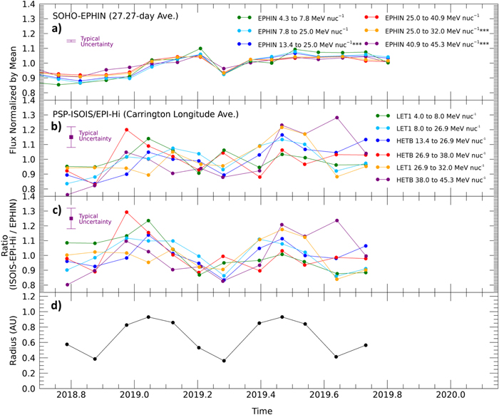
Figure 1. Evidence of a radial gradient in ACR helium observed by PSP/IS⊙IS after (i) subtracting out solar events, (ii) averaging out effects caused by solar wind streams, and (iii) correcting for changes in solar modulation. (a) 27.27 day averages of SOHO/EPHIN hourly fluxes, normalized by the mean for each energy band (derived from publicly available data: http://ulysses.physik.uni-kiel.de/costep/level3/l3i/) (b) IS⊙IS helium fluxes averaged over Carrington longitude (in the spacecraft frame), with energies binned and interpolated to match EPHIN. (c) IS⊙IS data detrended by taking the ratios of results at each energy (panel b) to their linearly interpolated EPHIN counterpart (from panel a). (d) PSP's radial distance from the Sun vs. time, with time-bins synchronized to that of EPI-Hi (b & c).
Download figure:
Standard image High-resolution imageNext, we examine the gradient more closely by applying fits to the different LET1 and HET B energy bands as a function of radial distance. To extract its magnitude, we perform least squares fits to the fluxes in linear space, assuming a differential radial gradient of the form:
(see, e.g., Jokipii 1971; Strauss & Potgieter 2010). Results are shown in Figure 2 and more details about our fitting process can be found in the Appendix.
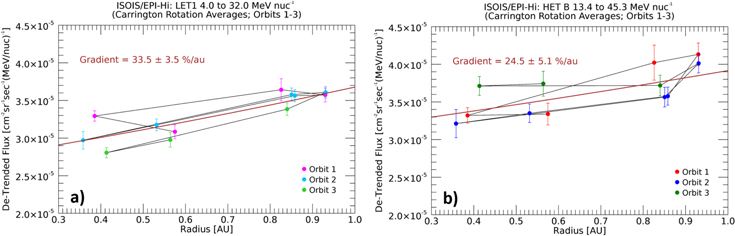
Figure 2. Carrington-averaged, detrended fluxes as a function of radius (see Figure 1) over (a) LET1's 4.0–32.0 MeV/nuc energy range and (b) HET B’s 13.4 to 45.3 MeV/nuc energy range. Collective fits yield gradients of 33.5 ± 3.5%/au and 24.5 ± 5.1%/au for LET1 and HET B, respectively.
Download figure:
Standard image High-resolution imageAlthough the method described so far (Method #1) minimizes the variations caused by solar wind streams, solar rotations in the PSP frame last anywhere from ∼27 to ∼47 days, which is longer than the typical time that the spacecraft spends under 0.25 au (∼10 days). As such, this long-term averaging will flatten some of the trend at smaller radii. We therefore explore two additional approaches of fitting: (a) to detrended daily averages 9 (Method #2; Figures 3(a) and (b)) and (b) to data that has been detrended and averaged over 0.01 au radial increments (Method #3; Figures 4(a) and (b)).
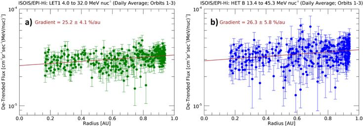
Figure 3. Flux vs. radius plots showing radial-gradient fits to daily averaged, detrended fluxes (Method #2) for (a) LET1 (25.2 ± 4.1%/au; 4.0 to 32.0 MeV/nuc) and (b) HET B (26.3 ± 5.8%/au; 13.4 to 45.3 MeV/nuc).
Download figure:
Standard image High-resolution image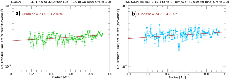
Figure 4. Flux vs. radius plots showing radial-gradient fits to radially binned, detrended fluxes (Method #3; 0.01-au increments) for (a) LET1 (23.8 ± 3.2%/au; 4.0 to 32.0 MeV/nuc) and (b) HET B (24.7 ± 4.7%/au; 13.4 to 45.3 MeV/nuc).
Download figure:
Standard image High-resolution imageResults from the three types of fits, and their dependence on energy, are summarized in Figure 5 and listed in Table 1 (Rankin et al., this study). In general, measurements by the two telescopes are consistent with each other and values achieved by the various methods exhibit reasonable agreement. For example, we report radial intensity gradients of 33.5 ± 3.5%/au, 25.2 ± 4.1%/au, and 23.8 ± 3.2%/au for helium energies of 4.0 to 32.0 MeV/nuc (LET1; Methods #1, #2, and #3, respectively), and 24.5 ± 5.1%/au, 26.3 ± 5.8%/au, and 24.7 ± 4.7%/au for energies of 13.4 to 45.3 MeV/nuc (HET B; same respective methods). These results are also compared with those of prior ACR helium studies, carried out during previous solar minima (Table 1).
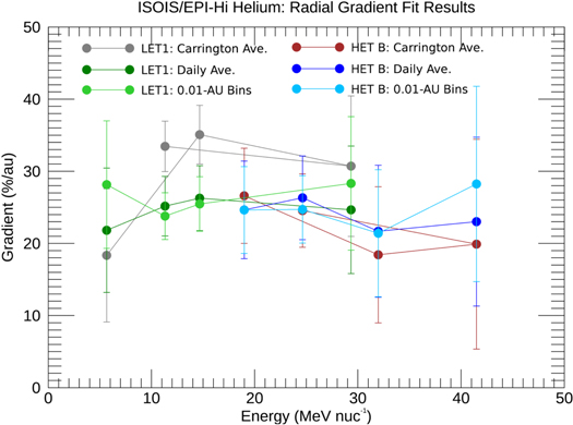
Figure 5. Radial gradients derived by applying three methods to IS⊙IS/EPI-Hi detrended, event-subtracted helium fluxes for the LET1 and HET B telescopes. Energies shown reflect the geometric means of the ranges reported in Table 1.
Download figure:
Standard image High-resolution imageTable 1. Radial Gradients of ACR Helium Over Various Solar Minima
| Reference | Time of Observation | Energy Range [MeV/nuc] | Gradient [%/au] | Solar Conditions | Spacecraft | Radial Distance [au] |
|---|---|---|---|---|---|---|
| Rankin et al. (this study) | 2018.7 to 2019.9 | 4.0 to 8.0 | 18.3 ± 9.2 | qA > 0 | PSP | 0.17 to 0.94 |
| Method #1 | 8.0 to 26.9 | 35.1 ± 4.1 | ||||
| (LET1) | 26.9 to 32.0 | 30.7 ± 9.7 | ||||
| 4.0 to 32.0 | 33.5 ± 3.5 | |||||
| Rankin et al. (this study) | 2018.7 to 2019.9 | 13.4 to 26.9 | 26.6 ± 6.6 | qA > 0 | PSP | 0.17 to 0.94 |
| Method #1 | 26.9 to 38.0 | 18.4 ± 9.4 | ||||
| (HET B) | 38.0 to 45.3 | 19.9 ± 14.5 | ||||
| 13.4 to 45.3 | 24.5 ± 5.1 | |||||
| Rankin et al. (this study) | 2018.7 to 2019.9 | 4.0 to 8.0 | 21.8 ± 8.6 | qA > 0 | PSP | 0.17 to 0.94 |
| Method #2 | 8.0 to 26.9 | 26.3 ± 4.5 | ||||
| (LET1) | 26.9 to 32.0 | 24.7 ± 8.8 | ||||
| 4.0 to 32.0 | 25.2 ± 4.1 | |||||
| Rankin et al. (this study) | 2018.7 to 2019.9 | 13.4 to 26.9 | 24.6 ± 6.8 | qA > 0 | PSP | 0.17 to 0.94 |
| Method #2 | 26.9 to 38.0 | 21.7 ± 9.1 | ||||
| (HET B) | 38.0 to 45.3 | 23.0 ± 11.7 | ||||
| 13.4 to 45.3 | 26.3 ± 5.8 | |||||
| Rankin et al. (this study) | 2018.7 to 2019.9 | 4.0 to 8.0 | 28.1 ± 8.8 | qA > 0 | PSP | 0.17 to 0.94 |
| Method #3 | 8.0 to 26.9 | 25.5 ± 3.8 | ||||
| (LET1) | 26.9 to 32.0 | 28.3 ± 9.3 | ||||
| 4.0 to 32.0 | 23.8 ± 3.2 | |||||
| Rankin et al. (this study) | 2018.7 to 2019.9 | 13.4 to 26.9 | 24.6 ± 6.0 | qA > 0 | PSP | 0.17 to 0.94 |
| Method #3 | 26.9 to 38.0 | 21.4 ± 8.8 | ||||
| (HET B) | 38.0 to 45.3 | 28.2 ± 13.5 | ||||
| 13.4 to 45.3 | 24.7 ± 4.7 | |||||
| Webber et al. (1981) | 1972 to 1978 | 10 to 21.6 | 15 ± 3 | qA > 0 | P10 | 3.0 to 14.8 |
| Bastian et al. (1981) | 1972 to 1977 | 11 to 20 | 14.3 ± 0.5 | qA > 0 | P10; I8 | 3.0 to 14.8; 1.0; ∼10 to ∼11 |
| 20.6 ± 0.9 | P11 ; I8 | |||||
| 10.5 ± 0.5 | P10; P11 | |||||
| Bastian et al. (1981) | 1972 to 1977 | 29 to 67 | 8.2 ± 0.3 | qA > 0 | P10; I8 P11; I8 P10; P11 | 3.0 to 14.8; 1.0; ∼10 to ∼11 |
| 9.9 ± 0.5 | ||||||
| 6.5 ± 0.3 | ||||||
| McKibben (1989) | 1973 to 1979 | 11 to 20 | 19.2 ± 1.9 | qA > 0 | P11; I8 | ∼2 to ∼12; 1.0; ∼4 to ∼31 |
| 11 to 20 | 11.4 ± 0.6 | P11; P10 | ||||
| 29 to 67 | 7.4 ± 0.9 | P11; I8 | ||||
| 29 to 67 | 4.7 ± 0.4 | P11; P10 | ||||
| McDonald & Lal (1987) | 1985.9 to 1986.1 | 10 to 21.7 | ∼4.7 | qA < 0 | P10; V2 | 18.9; 37.4 |
| 30 to 56 | ∼4.6 | |||||
| Cummings et al. (1987) | 1985.6 to 1986.2 | 10 to 21.7 | 5.3 ± 0.6 | qA < 0 | P10; V1; V2 | 36.9; 24.9, 18.4 |
| 30 to 56 | 5.0 ± 0.4 | P10; V1; V2 | ||||
| Cummings et al. (1990) | ∼1987 | 20 to 25 | ∼12% | qA < 0 | P10; P11; V1; V2; I8 | 40.7; 22.9; 29.9; 22.5; 1.0 |
| McDonald et al. (1997) | 1993 to 1996 | 30 to 60 | 22 ± 3 | qA > 0 | ULS; I8; V2 | 2.29 to 5.07; 1.0; 39.1 to 47.9 |
| McDonald et al. (2001) | 1996 to 2001.3 | 34 to 50 | ∼9.5 | qA > 0 | V1; V2; I8, ULS | 61.8 to 79.9; 47.8 to 62.8; 1.0; 2.02 to 5.37 |
Note. Results from this current study (Rankin et al. 2021) utilize PSP/IS⊙IS/EPI-Hi observations from 0.17 to 0.94 au during the ∼2018.7 to ∼2019.9 time period (orbits 1–3). These are derived from detrended, event-subtracted helium fluxes using three approaches: (i) fits to data averaged over Carrington longitude in the PSP frame to reduce effects caused by solar wind streams (Method #1), (ii) fits data averaged over 1 day time intervals (Method #2), and (iii) fits to data binned over 0.01 au radial increments (Method #3). Results from past studies were typically derived from multiple spacecraft arrayed at varying radial distances (and latitudes) in the inner heliosphere, including Pioneers 10 & 11 (P10; P11), Voyagers 1 & 2 (V1; V2), Ulysses (ULS), and IMP-8 (I8). Minima to date have occurred around ∼1973.2 (solar cycle 21), ∼1986.7 (solar cycle 22), ∼1996.6 (solar cycle 23), ∼2008.9 (solar cycle 24) and ∼2019.9 (solar cycle 25); see, e.g., Ross & Chaplin (2019).
Download table as: ASCIITypeset image
The gradients we measure are stronger than those reported by prior studies and unexpectedly large compared with the few measurements taken during qA < 0 periods. Observations reported by previous studies vary widely, probably due to their reliance on measurements from multiple spacecraft as well as out-of-the-ecliptic trajectories that can include a strong function of both radius and latitude. PSP's repeated coverage in radial distance at low-ecliptic latitudes is advantageous for continued study, particularly as the solar cycle progresses (see Guo et al. 2021 for details of PSP’s orbit). The interplay between drifts and diffusion in cosmic ray transport is not fully understood and the degree to which one or the other prevails as a function of time or location may also account for differences between our observations and those of previous studies. As drifts are mostly energy dependent and diffusion is typically assumed to depend on rigidity (atomic number per charge), continued observations with multiple species and longer accumulations of statistics should provide better insight into these processes inside 1 au.
Figure 6 presents simulated radial gradients of ACR helium in the equatorial plane as a function of kinetic energy for varying distances in the inner heliosphere. We use the model of Strauss & Potgieter (2010)—applied in that paper to ACR oxygen gradients—with some minor updates and modifications, including (i) a heliospheric current sheet tilt angle of 10° (a typical value chosen to reflect conditions during solar minimum), (ii) movement of the heliopause position to 120 au (to be consistent with Voyager observations), and (iii) the appropriate atomic number to charge ratio (A/Q = 4) for singly-charged helium. The fits we derive from the PSP measurements, along with their associated error bars, are superimposed in green.
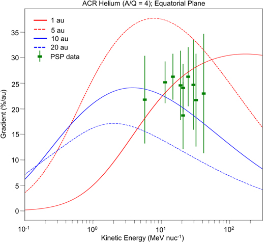
Figure 6. Simulated radial gradients of ACR helium in the equatorial plane as a function of kinetic energy for radial distances of 1 au (solid red line), 5 au (dashed red line), 10, au (solid blue line), and 20 au (dashed blue line). Values derived from PSP observations (green) compare relatively well with the values modeled at Earth (1 au; red solid line). Results are generated using the model of Strauss & Potgieter (2010), with minor updates.
Download figure:
Standard image High-resolution imageThe challenge of interpreting observed gradients over varying radial distances and as a function of energy is illustrated in Figure 6. Where the peak occurs as a function of energy depends on heliocentric distance, with the lowest energy peaks occurring at larger distances. This is not too surprising because higher energy particles are expected to penetrate deeper into the heliosphere. Even so, the 1-au curve, which best agrees with our data, predicts that we should observe the strongest gradient at even higher energies than we have examined in the present study. In contrast to traditional theory, the Strauss & Potgieter (2010) model predicts that modulation in the inner heliosphere may be more dependent on diffusion than on the drift cycle; such behavior could explain some of the differences among observations from prior studies listed above. Closer in to the Sun however, drifts are much larger so the gradients tend to increase, but without data inside 1 au to constrain the models, the location of that peak (in this case at 5 au) has not yet been accurately determined as it is a combination of the transport coefficients, the choice of the inner boundary condition, and other model-dependent parameters.
Overall, our initial comparison between simulated and measured radial gradients shows relatively good agreement with results at 1 au, but the applicability of traditional transport models inside 1 au is yet to be worked out in detail. One challenge presented by the PSP measurements is the choice of inner boundary condition when solving the isotropic Parker (1965) transport equation. Traditionally, these transport models implement a reflecting inner boundary condition inside 1 au which will lead to a zero radial gradient at that point (e.g., Jokipii et al. 1977; Siluszyk & Alania 2001; Strauss & Potgieter 2010). It is not yet clear how this should be treated; for example, cosmic rays could be increasingly mirrored as PSP approaches the Alfvénic point, leading to an increasingly anisotropic particle distribution and possibly invalidate the use of the Parker transport equation in this region.
Another way that our observations challenge current models relates to galactic cosmic rays (GCRs). GCR radial gradients are observed to be smaller than for ACRs—even of the same energy and species—owing to their steeper spectrum and fully ionized charge states (A/Q = 2 for GCRs versus A/Q = 4 for ACRs; recall that ACRs are singly ionized). PSP/IS⊙IS/EPI-Hi does not distinguish between charge states and thus subtracting out the GCR background requires a reliable model of the GCR spectrum. Even so, the modulated behavior of GCRs at their lowest energies (∼10 to ∼100 MeV/nuc; overlapping with ACRs) is highly model dependent, and very little observational data exists to provide inputs inside 1 au. A plot of the helium spectrum observed by PSP/IS⊙IS/EPI-Hi and SOHO/EPHIN is included in Figure 7 (see also the Appendix for further details). Superimposed is a simulation of the modulated GCR helium spectrum at 1 au (using the HelMod Online Calculator; version 4.0.1, 2021 January; www.helmod.org which indicates that GCRs could comprise as much as ∼25%–50% of the total intensity in the ∼15 to ∼40 MeV/nuc median energy range, simulated over the same time period as our data. Preliminary analysis shows that subtracting the GCR component and refitting to the remaining fluxes yields larger gradients than we previously derived. For example, using Method #2 we find: (a) 34.3 ± 5.6%/au for LET1 (4.0–32.0 MeV/nuc; increased from 25.2 ± 4.1%/au) and (b) 44.7 ± 10.2%/au for HET B (13.4 to 45.3 MeV/nuc; increased from 26.3 ± 5.8%/au); see the Appendix for more details. Consequently, the “ACR” radial gradients we report in this study serve as lower bounds because of the uncorrected GCR background. As GCR fluxes are expected to be smaller near the Sun than at 1 au and additional analysis (including that of protons) is needed to inform models and derive more accurate parameters in this new regime, we leave the more realistic corrections as a topic for future work.
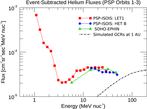
Figure 7. Event-subtracted helium fluxes measured by the PSP/IS⊙IS/EPI-Hi (LET1 in red; HET B in blue) and SOHO/EPHIN (green), over the fully calibrated energy ranges of their respective telescopes. Data in the ∼5 to ∼40 MeV/nuc range (median energies) were used for the current analysis of radial intensity gradients. Also included is the simulated GCR helium spectrum at 1 au (black), obtained using HelMod (version 4.0.1, 2021 January; www.helmod.org. Although the largest SEP events have been omitted, some particle increases due to CIRs may also be present and probably accounts for the turn-up in LET1 below a few MeV/nuc. However, as these do not contribute to the spectrum above ∼5 MeV, they do not affect the ACR measurements.
Download figure:
Standard image High-resolution imageA final aspect to consider in the interpretation of our results is the unusual properties of the magnetic field near the Sun. Drift, diffusion, and other terms that describe cosmic ray transport are dependent upon the magnitude of the heliospheric magnetic field, typically characterized by a radial component ∝1/R2 and a transverse component ∝1/R. In varying combinations, these are commonly used to calculate the Parker spiral field as a function of heliocentric distance for any solar wind speed. While the transverse term tends to dominate in the outer heliosphere, the opposite appears to be true inside 1 au—as the more radial field dominates over the cross-field diffusion, cosmic rays should gain better access closer to the Sun, as evidenced by our observations. Therefore, in addition to continued measurements with PSP/IS⊙IS, we need to take into account the real behavior of the magnetic field. In fact, it is not just the Parker spiral that should be considered; evidence suggests that Sub- and Super-Parker deviations arising from footpoint motion and interchange reconnection (Fisk 1996; Fisk et al. 1999; Fisk & Schwadron 2001) provide a magnetic connection of field lines across source regions of slow and fast solar wind, which may also be important for modeling cosmic ray transport near the Sun and in the inner heliosphere (Schwadron & McComas 2005, 2021).
In conclusion, PSP enables a new view of the propagation of particles into the plasma environment close to the Sun. Here, we have reported on the first observations of radial gradients of ACR helium all the way in to ∼36 solar radii (∼0.166 au). Not only are these the first measurements ever taken inside ∼0.3 au, but they are also the first during the minimum of the present solar cycle, at a time when IBEX has completed a full solar cycle of observations (McComas et al. 2020) and both Voyagers have crossed through the heliosheath and beyond the heliopause. Combined, these observations have led to significantly improved understanding of the pickup ions from which ACR’s are formed as well as of the large-scale structure of the heliosphere—understanding that was not present at the time of ACR discovery over 40 yr ago. Moreover, unlike in the past, there are currently no missions on escape trajectories within the heliosphere that are capable of measuring ACRs. Lastly, PSP's repeated sampling of the near-Sun environment over short timescales will enable an unprecedented glimpse of conditions as they evolve over the solar cycle. As such, continued measurements of ACRs on PSP (and Solar Orbiter) will play a critical role in linking past observations with our present knowledge and significantly advancing our understanding of cosmic ray transport in the inner heliosphere.
This work was supported as a part of the Integrated Science Investigation of the Sun on NASA’s Parker Solar Probe mission, under contract NNN06AA01C. The IS⊙IS data and visualization tools are available to the community at https://spacephysics.princeton.edu/missions-instruments/isois; data are also available via the NASA Space Physics Data Facility (https://spdf.gsfc.nasa.gov/). We thank the SOHO/EPHIN team at Christian-Albrechts-Universität zu Kiel for making their data publicly available and Patrick Kühl and Bernd Heber for their guidance as well as their thorough documentation of the level 3 data product. We also gratefully acknowledge the support provided by Michigan State University’s National Superconducting Cyclotron Laboratory, Texas A&M University’s Cyclotron Institute, and the Lawrence Berkeley National Laboratory’s 88 inch Cyclotron Laboratory during EPI-Hi’s calibration and testing. Parker Solar Probe was designed, built, and is now operated by the Johns Hopkins Applied Physics Laboratory as part of NASA’s Living with a Star (LWS) program. Support from the LWS management and technical team has played a critical role in the success of the Parker Solar Probe mission. We thank all the scientists and engineers who have worked hard to make PSP a successful mission.
A.1. Data Processing & Event Subtraction
Calibration efforts for IS⊙IS/EPI-Hi are ongoing, particularly for helium and the heavier elements. As such, there are several things we have taken into account in the selection of data presented here. First, as stated earlier in the main text, we use both the A- and B-sides of LET1 (averaged together), but only the B-side of HET because its quiet-time A-side rates are contaminated with background arising from partial obstruction by PSP's thermal protection system. Second, although HET’s energy range extends lower than 13.4 MeV/nuc, we presently omit its lowest energy channels as they too are dominated by background, though for different reasons than described above. Time periods when the helium fluxes are dominated by transient increases due to solar energetic particles or particles accelerated by stream interaction regions are omitted in this study (Tables 2 and 3). During these periods, the science rates are artificially high because they were not initialized to “0” following an instrument power-on. This issue no longer occurs after being fixed on board by a command, and such periods will be flagged or omitted in future versions of the released data.
Table 2. Time Periods Omitted from the LET1 Hourly Fluxes (See the Text)
| Year | Day of Year | Hour |
|---|---|---|
| 2018 | 241 | 6 |
| 2018 | 247 | 15 |
| 2018 | 247 | 17 |
| 2018 | 253 | 14 |
| 2018 | 253 | 15 |
| 2018 | 260 | 6 |
| 2018 | 267 | 21 |
| 2018 | 275 | 4 |
| 2018 | 276 | 2 |
| 2018 | 276 | 16 |
| 2018 | 281 | 16 |
| 2018 | 284 | 15 |
| 2018 | 287 | 14 |
| 2018 | 318 | 5 |
| 2018 | 342 | 14 |
| 2018 | 343 | 15 |
| 2018 | 344 | 15 |
| 2018 | 345 | 9 |
| 2018 | 345 | 21 |
| 2018 | 346 | 13 |
| 2018 | 346 | 21 |
| 2018 | 347 | 6 |
| 2018 | 347 | 15 |
| 2018 | 348 | 15 |
| 2018 | 348 | 22 |
| 2018 | 350 | 5 |
| 2019 | 1 | 12 |
| 2019 | 180 | 23 |
| 2019 | 250 | 11 |
| 2020 | 113 | 17 |
Download table as: ASCIITypeset image
Table 3. Time Periods Omitted from the HET Hourly Fluxes (See the Text)
| Year | Day of Year | Hour |
|---|---|---|
| 2018 | 241 | 6 |
| 2018 | 247 | 15 |
| 2018 | 253 | 14 |
| 2018 | 253 | 15 |
| 2018 | 260 | 6 |
| 2018 | 267 | 16 |
| 2018 | 279 | 7 |
| 2018 | 284 | 15 |
| 2018 | 345 | 9 |
| 2018 | 348 | 15 |
| 2019 | 205 | 16 |
| 2019 | 214 | 23 |
| 2019 | 220 | 14 |
| 2019 | 222 | 1 |
| 2019 | 253 | 8 |
| 2019 | 263 | 13 |
Download table as: ASCIITypeset image
Time periods when the He fluxes are dominated by transient increases due to solar energetic particles or particles accelerated by stream interaction regions are omitted in this study. This event subtraction is performed by using the hourly-averaged helium fluxes for both PSP/IS⊙IS/EPI-Hi and SOHO/EPHIN. We identify and subtract events for each data set independently (over each energy channel) via a simple algorithm as follows: (a) we first apply moving averages to smooth the data (∼5 to ∼11 hr, depending on the statistical limitations for a given channel), (b) we then select time periods when 5 or more consecutive points are at least 2-sigma above the mean, and (c) identify the start and end times of an “event” by tracking when its fluxes deviate/return to the mean. We apply this identification scheme for each separate energy band, but remove the identified events from all energies, even if they do not appear to be affected. For the most part, the algorithm appears to work reasonably well and there are encouraging commonalities that we find between the two spacecraft (see Table 5 for event list).
Although the time period considered in our study is, for the most part, relatively quiet, we have worked to establish a de-trending approach that will remain applicable in the future with more significant variations in the level of solar modulation. As EPI-Hi’s energy bins are much more finely spaced than EPHIN’s, we identify the ranges that best overlap and take the energy-weighted average:
For i energy bins, where x is the average for the new larger energy bin and fi (t) is the reported flux at some time t, with width △Ei . For the most part, EPHIN and IS⊙IS/EPI-Hi energy channels coincide quite well (Table 4). But, for those cases in which EPI-Hi’s channels do not fully overlap (e.g., HET’s lowest energies and LET1's highest), we extract the 1 au baseline fluxes by linearly interpolating the EPHIN data as a function of energy.
Table 4. Index of Relevant Energy Channels for SOHO/EPHIN and PSP/IS⊙IS/EPI-Hi Helium
| EPHIN Energy Channels [MeV/nuc] | IS⊙IS/EPI-Hi LET1 Energy Channels [MeV/nuc] | IS⊙IS/EPI-Hi HET Energy Channels [MeV/nuc] |
|---|---|---|
| 4.3 | 4.0 | NA |
| 4.8 | ||
| 5.7 | ||
| 6.7 | ||
| 7.8 | 8.0 | |
| 9.5 | ||
| 11.3 | ||
| 13.4 | 13.4 | |
| 16.0 | 16.0 | |
| 19.0 | 19.0 | |
| 22.6 | 22.6 | |
| 25.0 | 26.9 | 26.9 |
| 32.0 | 32.0 | |
| 40.9 | NA | 38.0 |
| 45.3 | ||
| 53.0 |
Download table as: ASCIITypeset image
Table 5. Helium “Event List” with Time Periods Identified and Subtracted Out from SOHO/EPHIN and PSP/IS⊙IS/EPI-Hi Helium Fluxes
| EPHIN | IS⊙IS/EPI-Hi | ||
|---|---|---|---|
| Start | End | Start | End |
| 2018.114 | 2018.125 | ⋯ | ⋯ |
| 2018.655 | 2018.67 | 2018.661 | 2018.696 |
| ⋯ | ⋯ | 2018.890 | 2018.900 |
| 2019.087 | 2019.091 | 2019.065 | 2019.078 |
| 2019.184 | 2019.186 | ⋯ | ⋯ |
| 2019.217 | 2019.222 | 2019.252 | 2019.270 |
| 2019.301 | 2019.307 | 2019.290 | 2019.311 |
| 2019.341 | 2019.351 | 2019.332 | 2019.354 |
Note. Time periods in bold are consistent with SEP events identified by Leske et al. (2020) and Wiedenbeck et al. (2020).
Download table as: ASCIITypeset image
A.2. Fitting Function
A generalized form of the total gradient can be derived from the cosmic ray transport equation (Parker 1965; Jokipii 1971) and is given by
where ,
, and
represent the radial, polar, and azimuthal unit vectors, respectively, and the individual components are defined as
for some differential intensity, j. PSP’s orbit varies only weakly in latitude, ranging from −41 to 41 in heliographic coordinates (necessitated by the Venus encounters; Guo et al. 2021), which is well below the tilt of the current sheet during this time (∼10° and larger; see, e.g., Wilcox Solar Observatory data: http://wso.stanford.edu/Tilts.html). As such, we ignore the latitudinal component in this study. We additionally assume that the gradient is independent of longitude (azimuth). This leaves us with a final term—the radial gradient (gr ). Translating from differential intensity to flux (j → f), yields:
which is the form that is the most applicable to our observations (see also Jokipii 1971; Jokipii et al. 1977 and Strauss & Potgieter 2010 for additional theoretical details). Although its solution is simply a linear equation in log space, we perform our fits in linear space to avoid the complications that arise from introducing asymmetric uncertainties. As such, we perform least squares fits to the fluxes as a function of radius using the simple relation: y = emx+B (flux y, radius x, gradient m), via the IDL-optimized MPFIT program (Markwardt 2009; https://pages.physics.wisc.edu/~craigm/idl/fitting.html).
A.3. Galactic Cosmic Rays and the Helium Energy Spectrum
Figure 7 shows the helium spectrum observed by PSP/IS⊙IS/EPI-Hi LET1 and HET B telescopes over their full energies, along with SOHO/EPHIN over its full energy range for the 2018 August 29 through 2019 November 15 time period (PSP orbits 1–3). A detection efficiency correction has been applied to the LET1 data to account for the misassignment of particles on board due to crosstalk into a guard detector. The correction was derived from a sample of telemetered data, from which we determined how many of the “bad” particles were misidentified at each energy. As this error produces an offset in flux that is constant over the time used in this analysis, its impact on the radial intensity gradient is expected to be negligible. The correction will be applied to subsequent public data releases. Also superimposed on Figure 7 is a simulation of the modulated GCR helium spectrum at 1 au, produced using the HelMod online calculator (version 4.0.1, 2021 January; www.helmod.org over the same time period as the data. HelMod uses a 2D Monte Carlo simulation to solve the Parker (1965) transport equation to simulate the modulation of cosmic rays through the heliosphere using data-driven Solar Wind parameters as inputs (Bobik et al. 2012; Boschini et al. 2020).
The fits reported in the main text were performed using the total spectrum, which included GCRs. However, we can correct for the GCR background by subtracting the PSP/IS⊙IS/EPI-Hi fluxes at each energy bin from the interpolated value predicted by HelMod. In re-performing the flux versus radial distance fits to daily averages (Method #2), we obtain gradients that are much larger than previous values: (a) 34.3 ± 5.6%/au for LET1 (4.0–32.0 MeV/nuc; increased from 25.2 ± 4.1%/au) and (b) 44.7 ± 10.2%/au for HET (13.4–45.3 MeV/nuc; increased from 26.3 ± 5.8%/au).