This glossary defines artificial intelligence terms.
A
ablation
A technique for evaluating the importance of a feature or component by temporarily removing it from a model. You then retrain the model without that feature or component, and if the retrained model performs significantly worse, then the removed feature or component was likely important.
For example, suppose you train a classification model on 10 features and achieve 88% precision on the test set. To check the importance of the first feature, you can retrain the model using only the nine other features. If the retrained model performs significantly worse (for instance, 55% precision), then the removed feature was probably important. Conversely, if the retrained model performs equally well, then that feature was probably not that important.
Ablation can also help determine the importance of:
- Larger components, such as an entire subsystem of a larger ML system
- Processes or techniques, such as a data preprocessing step
In both cases, you would observe how the system's performance changes (or doesn't change) after you've removed the component.
A/B testing
A statistical way of comparing two (or more) techniques—the A and the B. Typically, the A is an existing technique, and the B is a new technique. A/B testing not only determines which technique performs better but also whether the difference is statistically significant.
A/B testing usually compares a single metric on two techniques; for example, how does model accuracy compare for two techniques? However, A/B testing can also compare any finite number of metrics.
accelerator chip
#GoogleCloud
A category of specialized hardware components designed to perform key computations needed for deep learning algorithms.
Accelerator chips (or just accelerators, for short) can significantly increase the speed and efficiency of training and inference tasks compared to a general-purpose CPU. They are ideal for training neural networks and similar computationally intensive tasks.
Examples of accelerator chips include:
- Google's Tensor Processing Units (TPUs) with dedicated hardware for deep learning.
- NVIDIA's GPUs which, though initially designed for graphics processing, are designed to enable parallel processing, which can significantly increase processing speed.
accuracy
#fundamentals
#Metric
The number of correct classification predictions divided by the total number of predictions. That is:
$$\text{Accuracy} = \frac{\text{correct predictions}} {\text{correct predictions + incorrect predictions }}$$
For example, a model that made 40 correct predictions and 10 incorrect predictions would have an accuracy of:
$$\text{Accuracy} = \frac{\text{40}} {\text{40 + 10}} = \text{80%}$$
Binary classification provides specific names for the different categories of correct predictions and incorrect predictions. So, the accuracy formula for binary classification is as follows:
$$\text{Accuracy} = \frac{\text{TP} + \text{TN}} {\text{TP} + \text{TN} + \text{FP} + \text{FN}}$$
where:
- TP is the number of true positives (correct predictions).
- TN is the number of true negatives (correct predictions).
- FP is the number of false positives (incorrect predictions).
- FN is the number of false negatives (incorrect predictions).
Compare and contrast accuracy with precision and recall.
Click the icon for details about accuracy and class-imbalanced datasets.
Although a valuable metric for some situations, accuracy is highly misleading for others. Notably, accuracy is usually a poor metric for evaluating classification models that process class-imbalanced datasets.
For example, suppose snow falls only 25 days per century in a certain subtropical city. Since days without snow (the negative class) vastly outnumber days with snow (the positive class), the snow dataset for this city is class-imbalanced. Imagine a binary classification model that is supposed to predict either snow or no snow each day but simply predicts "no snow" every day. This model is highly accurate but has no predictive power. The following table summarizes the results for a century of predictions:
| Category | Number |
|---|---|
| TP | 0 |
| TN | 36499 |
| FP | 0 |
| FN | 25 |
The accuracy of this model is therefore:
accuracy = (TP + TN) / (TP + TN + FP + FN)
accuracy = (0 + 36499) / (0 + 36499 + 0 + 25) = 0.9993 = 99.93%
Although 99.93% accuracy seems like a very impressive percentage, the model actually has no predictive power.
Precision and recall are usually more useful metrics than accuracy for evaluating models trained on class-imbalanced datasets.
See Classification: Accuracy, recall, precision and related metrics in Machine Learning Crash Course for more information.
act
#agent
A stage in the agentic loop in which the agent executes the action chosen during the reason stage. For example, the act stage could send an API request.
action
#agent
In reinforcement learning, the mechanism by which the agent transitions between states of the environment. The agent chooses the action by using a policy.
action space
#agent
The set of resources an agent can use to perform a task. Action space might include the tools and APIs that the agent can invoke and the permissions the agent holds. In general, the action space should be just big enough for the agent to perform the task. If the action space is too small, the agent might have insufficient resources to perform the task. If the action space is too large, the agent tends to become more error prone.
activation function
#fundamentals
A function that enables neural networks to learn nonlinear (complex) relationships between features and the label.
Popular activation functions include:
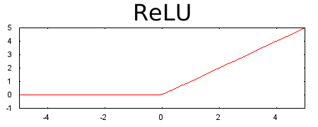
The plots of activation functions are never single straight lines. For example, the plot of the ReLU activation function consists of two straight lines:
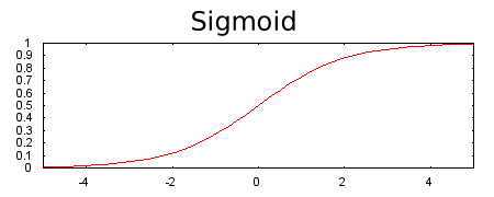
A plot of the sigmoid activation function looks as follows:
Click the icon to see an example.
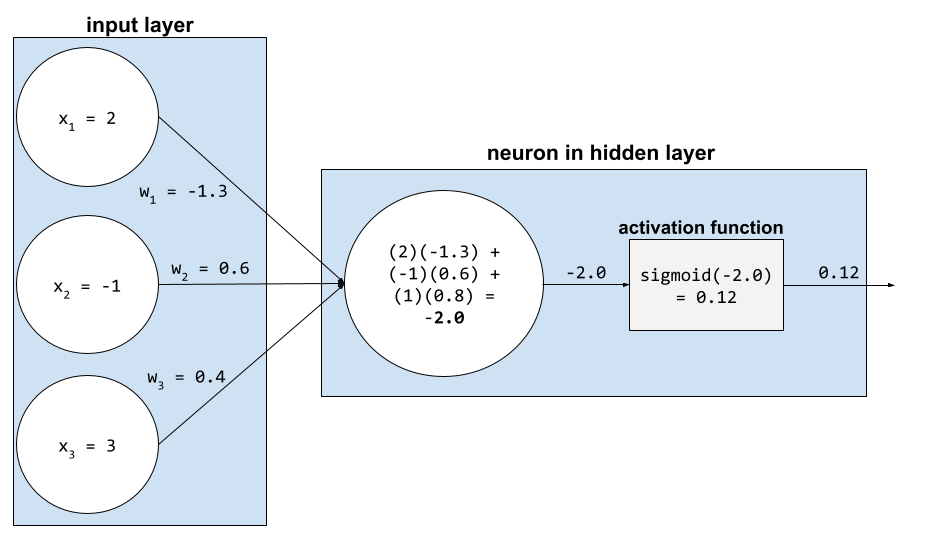
In a neural network, activation functions manipulate the weighted sum of all the inputs to a neuron. To calculate a weighted sum, the neuron adds up the products of the relevant values and weights. For example, suppose the relevant input to a neuron consists of the following:
| input value | input weight |
| 2 | -1.3 |
| -1 | 0.6 |
| 3 | 0.4 |
The weighted sum is therefore:
weighted sum = (2)(-1.3) + (-1)(0.6) + (3)(0.4) = -2.0
Suppose the designer of this neural network chooses the sigmoid function to be the activation function. In that case, the neuron calculates the sigmoid of -2.0, which is approximately 0.12. Therefore, the neuron passes 0.12 (rather than -2.0) to the next layer in the neural network. The following figure illustrates the relevant part of the process:
See Neural networks: Activation functions in Machine Learning Crash Course for more information.
active learning
A training approach in which the algorithm chooses some of the data it learns from. Active learning is particularly valuable when labeled examples are scarce or expensive to obtain. Instead of blindly seeking a diverse range of labeled examples, an active learning algorithm selectively seeks the particular range of examples it needs for learning.
AdaGrad
A sophisticated gradient descent algorithm that rescales the gradients of each parameter, effectively giving each parameter an independent learning rate. For a full explanation, see Adaptive Subgradient Methods for Online Learning and Stochastic Optimization.
adaptation
#generativeAI
Synonym for tuning or fine-tuning.
agent
#generativeAI
#agent
Software that can reason about user inputs in order to plan and execute actions on behalf of the user.
In reinforcement learning, an agent is the entity that uses a policy to maximize the expected return gained from transitioning between states of the environment.
agentic
#generativeAI
#agent
The adjective form of agent. Agentic refers to the qualities that agents possess (such as autonomy).
agentic loop
#agent
A cycle that an agent iterates through until a termination condition is met. The cycle typically consists of the following four stages:
agentic workflow
#generativeAI
#agent
A dynamic process in which an agent autonomously plans and executes actions to achieve a goal. The process may involve reasoning, invoking external tools, and self-correcting its plan.
agent orchestration
#agent
The centralized management and routing of tasks across multiple sub-agents or LLM calls. Agent orchestration breaks down complex tasks into smaller sub-tasks and assigns them to the most capable sub-agents.
agglomerative clustering
#clustering
AI slop
#generativeAI
Output from a generative AI system that favors quantity over quality. For example, a web page with AI slop is filled with cheaply produced, AI-generated, low-quality content.
anomaly detection
The process of identifying outliers. For example, if the mean for a certain feature is 100 with a standard deviation of 10, then anomaly detection should flag a value of 200 as suspicious.
AR
Abbreviation for augmented reality.
area under the PR curve
#Metric
See PR AUC (Area under the PR Curve).
area under the ROC curve
#Metric
See AUC (Area under the ROC curve).
artificial general intelligence
A non-human mechanism that demonstrates a broad range of problem solving, creativity, and adaptability. For example, a program demonstrating artificial general intelligence could translate text, compose symphonies, and excel at games that have not yet been invented.
artificial intelligence
#fundamentals
A non-human program or model that can solve sophisticated tasks. For example, a program or model that translates text or a program or model that identifies diseases from radiologic images both exhibit artificial intelligence.
Formally, machine learning is a sub-field of artificial intelligence. However, in recent years, some organizations have begun using the terms artificial intelligence and machine learning interchangeably.
attention
A mechanism used in a neural network that indicates the importance of a particular word or part of a word. Attention compresses the amount of information a model needs to predict the next token/word. A typical attention mechanism might consist of a weighted sum over a set of inputs, where the weight for each input is computed by another part of the neural network.
Refer also to self-attention and multi-head self-attention, which are the building blocks of Transformers.
See LLMs: What's a large language model? in Machine Learning Crash Course for more information about self-attention.
attribute
#responsible
Synonym for feature.
In machine learning fairness, attributes often refer to characteristics pertaining to individuals.
attribute sampling
#df
A tactic for training a decision forest in which each decision tree considers only a random subset of possible features when learning the condition. Generally, a different subset of features is sampled for each node. In contrast, when training a decision tree without attribute sampling, all possible features are considered for each node.
AUC (Area under the ROC curve)
#fundamentals
#Metric
A number between 0.0 and 1.0 representing a binary classification model's ability to separate positive classes from negative classes. The closer the AUC is to 1.0, the better the model's ability to separate classes from each other.
For example, the following illustration shows a classification model that separates positive classes (green ovals) from negative classes (purple rectangles) perfectly. This unrealistically perfect model has an AUC of 1.0:

Conversely, the following illustration shows the results for a classification model that generated random results. This model has an AUC of 0.5:

Yes, the preceding model has an AUC of 0.5, not 0.0.
Most models are somewhere between the two extremes. For instance, the following model separates positives from negatives somewhat, and therefore has an AUC somewhere between 0.5 and 1.0:

AUC ignores any value you set for classification threshold. Instead, AUC considers all possible classification thresholds.
Click the icon to learn about the relationship between AUC and ROC curves.
AUC represents the area under an ROC curve. For example, the ROC curve for a model that perfectly separates positives from negatives looks as follows:
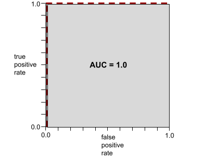
AUC is the area of the gray region in the preceding illustration. In this unusual case, the area is simply the length of the gray region (1.0) multiplied by the width of the gray region (1.0). So, the product of 1.0 and 1.0 yields an AUC of exactly 1.0, which is the highest possible AUC score.
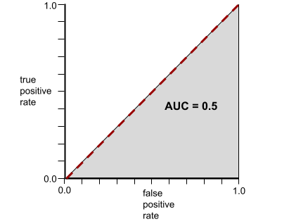
Conversely, the ROC curve for a classification model that can't separate classes at all is as follows. The area of this gray region is 0.5.
A more typical ROC curve looks approximately like the following:
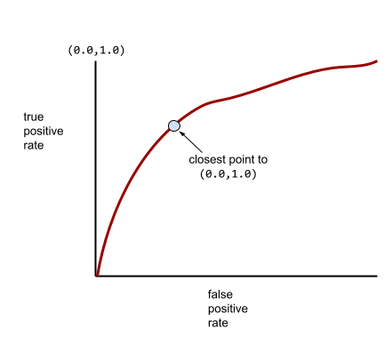
It would be painstaking to calculate the area under this curve manually, which is why a program typically calculates most AUC values.
Click the icon for a more formal definition of AUC.
AUC is the probability that a classification model will be more confident that a randomly chosen positive example is actually positive than that a randomly chosen negative example is positive.
See Classification: ROC and AUC in Machine Learning Crash Course for more information.
augmented reality
A technology that superimposes a computer-generated image on a user's view of the real world, thus providing a composite view.
autoencoder
A system that learns to extract the most important information from the input. Autoencoders are a combination of an encoder and decoder. Autoencoders rely on the following two-step process:
- The encoder maps the input to a (typically) lossy lower-dimensional (intermediate) format.
- The decoder builds a lossy version of the original input by mapping the lower-dimensional format to the original higher-dimensional input format.
Autoencoders are trained end-to-end by having the decoder attempt to reconstruct the original input from the encoder's intermediate format as closely as possible. Because the intermediate format is smaller (lower-dimensional) than the original format, the autoencoder is forced to learn what information in the input is essential, and the output won't be perfectly identical to the input.
For example:
- If the input data is a graphic, the non-exact copy would be similar to the original graphic, but somewhat modified. Perhaps the non-exact copy removes noise from the original graphic or fills in some missing pixels.
- If the input data is text, an autoencoder would generate new text that mimics (but is not identical to) the original text.
See also variational autoencoders.
automatic evaluation
#generativeAI
Using software to judge the quality of a model's output.
When model output is relatively straightforward, a script or program can compare the model's output to a golden response. This type of automatic evaluation is sometimes called programmatic evaluation. Metrics such as ROUGE or BLEU are often useful for programmatic evaluation.
When model output is complex or has no one right answer, a separate ML program called an autorater sometimes performs the automatic evaluation.
Contrast with human evaluation.
automation bias
#responsible
When a human decision maker favors recommendations made by an automated decision-making system over information made without automation, even when the automated decision-making system makes errors.
See Fairness: Types of bias in Machine Learning Crash Course for more information.
AutoML
Any automated process for building machine learning models. AutoML can automatically do tasks such as the following:
- Search for the most appropriate model.
- Tune hyperparameters.
- Prepare data (including performing feature engineering).
- Deploy the resulting model.
AutoML is useful for data scientists because it can save them time and effort in developing machine learning pipelines and improve prediction accuracy. It is also useful to non-experts, by making complicated machine learning tasks more accessible to them.
See Automated Machine Learning (AutoML) in Machine Learning Crash Course for more information.
autonomous agent
#agent
An agent that works towards a complex goal by planning, acting, and adapting without continuous human intervention.
autorater evaluation
#generativeAI
A hybrid mechanism for judging the quality of a generative AI model's output that combines human evaluation with automatic evaluation. An autorater is an ML model trained on data created by human evaluation. Ideally, an autorater learns to mimic a human evaluator.
Prebuilt autoraters are available, but the best autoraters are fine-tuned specifically to the task you are evaluating.
auto-regressive model
#generativeAI
A model that infers a prediction based on its own previous predictions. For example, auto-regressive language models predict the next token based on the previously predicted tokens. All Transformer-based large language models are auto-regressive.
In contrast, GAN-based image models are usually not auto-regressive since they generate an image in a single forward-pass and not iteratively in steps. However, certain image generation models are auto-regressive because they generate an image in steps.
auxiliary loss
A loss function—used in conjunction with a neural network model's main loss function—that helps accelerate training during the early iterations when weights are randomly initialized.
Auxiliary loss functions push effective gradients to the earlier layers. This facilitates convergence during training by combating the vanishing gradient problem.
average precision at k
#Metric
A metric for summarizing a model's performance on a single prompt that generates ranked results, such as a numbered list of book recommendations. Average precision at k is, well, the average of the precision at k values for each relevant result. The formula for average precision at k is therefore:
\[{\text{average precision at k}} = \frac{1}{n} \sum_{i=1}^n {\text{precision at k for each relevant item} } \]
where:
- \(n\) is the number of relevant items in the list.
Contrast with recall at k.
Click the icon for an example
Suppose a large language model is given the following query:
List the 6 funniest movies of all time in order.
And the large language model returns the following list:
- The General
- Mean Girls
- Platoon
- Bridesmaids
- Citizen Kane
- This is Spinal Tap
Four of the movies in the returned list are very funny (that is, they are relevant) but two movies are dramas (not relevant). The following table details the results:
| Position | Movie | Relevant? | Precision at k |
|---|---|---|---|
| 1 | The General | Yes | 1.0 |
| 2 | Mean Girls | Yes | 1.0 |
| 3 | Platoon | No | not relevant |
| 4 | Bridesmaids | Yes | 0.75 |
| 5 | Citizen Kane | No | not relevant |
| 6 | This is Spinal Tap | Yes | 0.67 |
The number of relevant results is 4. Therefore, you can calculate the average precision at 6 as follows:
$${\text{average precision at 6}} = \frac{1}{4} {\text{(1.0 + 1.0 + 0.75 + 0.67)} } $$ $${\text{average precision at 6}} = {\text{~0.85} } $$
axis-aligned condition
#df
In a decision tree, a condition
that involves only a single feature. For example, if area
is a feature, then the following is an axis-aligned condition:
area > 200
Contrast with oblique condition.
B
backpropagation
#fundamentals
The algorithm that implements gradient descent in neural networks.
Training a neural network involves many iterations of the following two-pass cycle:
- During the forward pass, the system processes a batch of examples to yield prediction(s). The system compares each prediction to each label value. The difference between the prediction and the label value is the loss for that example. The system aggregates the losses for all the examples to compute the total loss for the current batch.
- During the backward pass (backpropagation), the system reduces loss by adjusting the weights of all the neurons in all the hidden layer(s).
Neural networks often contain many neurons across many hidden layers. Each of those neurons contribute to the overall loss in different ways. Backpropagation determines whether to increase or decrease the weights applied to particular neurons.
The learning rate is a multiplier that controls the degree to which each backward pass increases or decreases each weight. A large learning rate will increase or decrease each weight more than a small learning rate.
In calculus terms, backpropagation implements the chain rule. from calculus. That is, backpropagation calculates the partial derivative of the error with respect to each parameter.
Years ago, ML practitioners had to write code to implement backpropagation. Modern ML APIs like Keras now implement backpropagation for you. Phew!
See Neural networks in Machine Learning Crash Course for more information.
bagging
#df
A method to train an ensemble where each constituent model trains on a random subset of training examples sampled with replacement. For example, a random forest is a collection of decision trees trained with bagging.
The term bagging is short for bootstrap aggregating.
See Random forests in the Decision Forests course for more information.
bag of words
A representation of the words in a phrase or passage, irrespective of order. For example, bag of words represents the following three phrases identically:
- the dog jumps
- jumps the dog
- dog jumps the
Each word is mapped to an index in a sparse vector, where the vector has an index for every word in the vocabulary. For example, the phrase the dog jumps is mapped into a feature vector with non-zero values at the three indexes corresponding to the words the, dog, and jumps. The non-zero value can be any of the following:
- A 1 to indicate the presence of a word.
- A count of the number of times a word appears in the bag. For example, if the phrase were the maroon dog is a dog with maroon fur, then both maroon and dog would be represented as 2, while the other words would be represented as 1.
- Some other value, such as the logarithm of the count of the number of times a word appears in the bag.
baseline
#Metric
A model used as a reference point for comparing how well another model (typically, a more complex one) is performing. For example, a logistic regression model might serve as a good baseline for a deep model.
For a particular problem, the baseline helps model developers quantify the minimal expected performance that a new model must achieve for the new model to be useful.
base model
#generativeAI
A pre-trained model that can serve as the starting point for fine-tuning to address specific tasks or applications.
See also pre-trained model and foundation model.
batch
#fundamentals
The set of examples used in one training iteration. The batch size determines the number of examples in a batch.
See epoch for an explanation of how a batch relates to an epoch.
See Linear regression: Hyperparameters in Machine Learning Crash Course for more information.
batch inference
#GoogleCloud
The process of inferring predictions on multiple unlabeled examples divided into smaller subsets ("batches").
Batch inference can take advantage of the parallelization features of accelerator chips. That is, multiple accelerators can simultaneously infer predictions on different batches of unlabeled examples, dramatically increasing the number of inferences per second.
See Production ML systems: Static versus dynamic inference in Machine Learning Crash Course for more information.
batch normalization
Normalizing the input or output of the activation functions in a hidden layer. Batch normalization can provide the following benefits:
- Make neural networks more stable by protecting against outlier weights.
- Enable higher learning rates, which can speed training.
- Reduce overfitting.
batch size
#fundamentals
The number of examples in a batch. For instance, if the batch size is 100, then the model processes 100 examples per iteration.
The following are popular batch size strategies:
- Stochastic Gradient Descent (SGD), in which the batch size is 1.
- Full batch, in which the batch size is the number of examples in the entire training set. For instance, if the training set contains a million examples, then the batch size would be a million examples. Full batch is usually an inefficient strategy.
- mini-batch in which the batch size is usually between 10 and 1000. Mini-batch is usually the most efficient strategy.
See the following for more information:
- Production ML systems: Static versus dynamic inference in Machine Learning Crash Course.
- Deep Learning Tuning Playbook.
Bayesian neural network
A probabilistic neural network that accounts for uncertainty in weights and outputs. A standard neural network regression model typically predicts a scalar value; for example, a standard model predicts a house price of 853,000. In contrast, a Bayesian neural network predicts a distribution of values; for example, a Bayesian model predicts a house price of 853,000 with a standard deviation of 67,200.
A Bayesian neural network relies on Bayes' Theorem to calculate uncertainties in weights and predictions. A Bayesian neural network can be useful when it is important to quantify uncertainty, such as in models related to pharmaceuticals. Bayesian neural networks can also help prevent overfitting.
Bayesian optimization
A probabilistic regression model technique for optimizing computationally expensive objective functions by instead optimizing a surrogate that quantifies the uncertainty using a Bayesian learning technique. Since Bayesian optimization is itself very expensive, it is usually used to optimize expensive-to-evaluate tasks that have a small number of parameters, such as selecting hyperparameters.
Bellman equation
In reinforcement learning, the following identity satisfied by the optimal Q-function:
\[Q(s, a) = r(s, a) + \gamma \mathbb{E}_{s'|s,a} \max_{a'} Q(s', a')\]
Reinforcement learning algorithms apply this identity to create Q-learning using the following update rule:
\[Q(s,a) \gets Q(s,a) + \alpha \left[r(s,a) + \gamma \displaystyle\max_{\substack{a_1}} Q(s',a') - Q(s,a) \right] \]
Beyond reinforcement learning, the Bellman equation has applications to dynamic programming. See the Wikipedia entry for Bellman equation.
BERT (Bidirectional Encoder Representations from Transformers)
A model architecture for text representation. A trained BERT model can act as part of a larger model for text classification or other ML tasks.
BERT has the following characteristics:
- Uses the Transformer architecture, and therefore relies on self-attention.
- Uses the encoder part of the Transformer. The encoder's job is to produce good text representations, rather than to perform a specific task like classification.
- Is bidirectional.
- Uses masking for unsupervised training.
BERT's variants include:
See Open Sourcing BERT: State-of-the-Art Pre-training for Natural Language Processing for an overview of BERT.
bias (ethics/fairness)
#responsible
#fundamentals
1. Stereotyping, prejudice or favoritism towards some things, people, or groups over others. These biases can affect collection and interpretation of data, the design of a system, and how users interact with a system. Forms of this type of bias include:
- automation bias
- confirmation bias
- experimenter's bias
- group attribution bias
- implicit bias
- in-group bias
- out-group homogeneity bias
2. Systematic error introduced by a sampling or reporting procedure. Forms of this type of bias include:
Not to be confused with the bias term in machine learning models or prediction bias.
See Fairness: Types of bias in Machine Learning Crash Course for more information.
bias (math) or bias term
#fundamentals
An intercept or offset from an origin. Bias is a parameter in machine learning models, which is symbolized by either of the following:
- b
- w0
For example, bias is the b in the following formula:
$$y' = b + w_1x_1 + w_2x_2 + … w_nx_n$$
In a simple two-dimensional line, bias just means "y-intercept." For example, the bias of the line in the following illustration is 2.
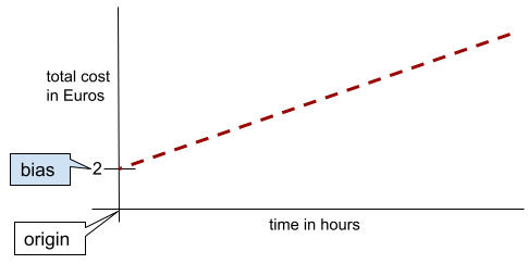
Bias exists because not all models start from the origin (0,0). For example, suppose an amusement park costs 2 Euros to enter and an additional 0.5 Euro for every hour a customer stays. Therefore, a model mapping the total cost has a bias of 2 because the lowest cost is 2 Euros.
Bias is not to be confused with bias in ethics and fairness or prediction bias.
See Linear Regression in Machine Learning Crash Course for more information.
bidirectional
A term used to describe a system that evaluates the text that both precedes and follows a target section of text. In contrast, a unidirectional system only evaluates the text that precedes a target section of text.
For example, consider a masked language model that must determine probabilities for the word or words representing the underline in the following question:
What is the _____ with you?
A unidirectional language model would have to base its probabilities only on the context provided by the words "What", "is", and "the". In contrast, a bidirectional language model could also gain context from "with" and "you", which might help the model generate better predictions.
bidirectional language model
A language model that determines the probability that a given token is present at a given location in an excerpt of text based on the preceding and following text.
bigram
An N-gram in which N=2.
binary classification
#fundamentals
A type of classification task that predicts one of two mutually exclusive classes:
- the positive class
- the negative class
For example, the following two machine learning models each perform binary classification:
- A model that determines whether email messages are spam (the positive class) or not spam (the negative class).
- A model that evaluates medical symptoms to determine whether a person has a particular disease (the positive class) or doesn't have that disease (the negative class).
Contrast with multi-class classification.
See also logistic regression and classification threshold.
See Classification in Machine Learning Crash Course for more information.
binary condition
#df
In a decision tree, a condition that has only two possible outcomes, typically yes or no. For example, the following is a binary condition:
temperature >= 100
Contrast with non-binary condition.
See Types of conditions in the Decision Forests course for more information.
binning
Synonym for bucketing.
black box model
A model whose "reasoning" is impossible or difficult for humans to understand. That is, although humans can see how prompts affect responses, humans can't determine exactly how a black box model determines the response. In other words, a black box model is lacking interpretability.
Most deep models and large language models are black boxes.
BLEU (Bilingual Evaluation Understudy)
A metric between 0.0 and 1.0 for evaluating machine translations, for example, from Spanish to Japanese.
To calculate a score, BLEU typically compares an ML model's translation (generated text) to a human expert's translation (reference text). The degree to which N-grams in the generated text and reference text match determines the BLEU score.
The original paper on this metric is BLEU: a Method for Automatic Evaluation of Machine Translation.
See also BLEURT.
BLEURT (Bilingual Evaluation Understudy from Transformers)
A metric for evaluating machine translations from one language to another, particularly to and from English.
For translations to and from English, BLEURT aligns more closely to human ratings than BLEU. Unlike BLEU, BLEURT emphasizes semantic (meaning) similarities and can accommodate paraphrasing.
BLEURT relies on a pre-trained large language model (BERT to be exact) that is then fine-tuned on text from human translators.
The original paper on this metric is BLEURT: Learning Robust Metrics for Text Generation.
Boolean Questions (BoolQ)
#Metric
A dataset for evaluating an LLM's proficiency in answering yes-or-no questions. Each of the challenges in the dataset has three components:
- A query
- A passage implying the answer to the query.
- The correct answer, which is either yes or no.
For example:
- Query: Are there any nuclear power plants in Michigan?
- Passage: ...three nuclear power plants supply Michigan with about 30% of its electricity.
- Correct answer: Yes
Researchers gathered the questions from anonymized, aggregated Google Search queries and then used Wikipedia pages to ground the information.
For more information, see BoolQ: Exploring the Surprising Difficulty of Natural Yes/No Questions.
BoolQ is a component of the SuperGLUE ensemble.
BoolQ
#Metric
Abbreviation for Boolean Questions.
boosting
A machine learning technique that iteratively combines a set of simple and not very accurate classification models (referred to as "weak classifiers") into a classification model with high accuracy (a "strong classifier") by upweighting the examples that the model is currently misclassifying.
See Gradient Boosted Decision Trees? in the Decision Forests course for more information.
bounding box
In an image, the (x, y) coordinates of a rectangle around an area of interest, such as the dog in the image below.

broadcasting
Expanding the shape of an operand in a matrix math operation to dimensions compatible for that operation. For example, linear algebra requires that the two operands in a matrix addition operation must have the same dimensions. Consequently, you can't add a matrix of shape (m, n) to a vector of length n. Broadcasting enables this operation by virtually expanding the vector of length n to a matrix of shape (m, n) by replicating the same values down each column.
Click the icon for an example.
Given the following definitions of A and B, linear algebra prohibits A+B because A and B have different dimensions:
A = [[7, 10, 4],
     [13, 5, 9]]
B = [2]
However, broadcasting enables the operation A+B by virtually expanding B to:
 [[2, 2, 2],
  [2, 2, 2]]
Thus, A+B is now a valid operation:
[[7, 10, 4],  +  [[2, 2, 2],  =  [[ 9, 12, 6],
 [13, 5, 9]]      [2, 2, 2]]      [15, 7, 11]]
See the following description of broadcasting in NumPy for more details.
bucketing
#fundamentals
Converting a single feature into multiple binary features called buckets or bins, typically based on a value range. The chopped feature is typically a continuous feature.
For example, instead of representing temperature as a single continuous floating-point feature, you could chop ranges of temperatures into discrete buckets, such as:
- <= 10 degrees Celsius would be the "cold" bucket.
- 11 - 24 degrees Celsius would be the "temperate" bucket.
- >= 25 degrees Celsius would be the "warm" bucket.
The model will treat every value in the same bucket identically. For
example, the values 13 and 22 are both in the temperate bucket, so the
model treats the two values identically.
Click the icon for additional notes.
If you represent temperature as a continuous feature, then the model treats temperature as a single feature. If you represent temperature as three buckets, then the model treats each bucket as a separate feature. That is, a model can learn separate relationships of each bucket to the label. For example, a linear regression model can learn separate weights for each bucket.
Increasing the number of buckets makes your model more complicated by increasing the number of relationships that your model must learn. For example, the cold, temperate, and warm buckets are essentially three separate features for your model to train on. If you decide to add two more buckets--for example, freezing and hot--your model would now have to train on five separate features.
How do you know how many buckets to create, or what the ranges for each bucket should be? The answers typically require a fair amount of experimentation.
See Numerical data: Binning in Machine Learning Crash Course for more information.
C
calibration layer
A post-prediction adjustment, typically to account for prediction bias. The adjusted predictions and probabilities should match the distribution of an observed set of labels.
candidate generation
The initial set of recommendations chosen by a recommendation system. For example, consider a bookstore that offers 100,000 titles. The candidate generation phase creates a much smaller list of suitable books for a particular user, say 500. But even 500 books is way too many to recommend to a user. Subsequent, more expensive, phases of a recommendation system (such as scoring and re-ranking) reduce those 500 to a much smaller, more useful set of recommendations.
See Candidate generation overview in the Recommendation Systems course for more information.
candidate sampling
A training-time optimization that calculates a probability for all the positive labels, using, for example, softmax, but only for a random sample of negative labels. For instance, given an example labeled beagle and dog, candidate sampling computes the predicted probabilities and corresponding loss terms for:
- beagle
- dog
- a random subset of the remaining negative classes (for example, cat, lollipop, fence).
The idea is that the negative classes can learn from less frequent negative reinforcement as long as positive classes always get proper positive reinforcement, and this is indeed observed empirically.
Candidate sampling is more computationally efficient than training algorithms that compute predictions for all negative classes, particularly when the number of negative classes is very large.
categorical data
#fundamentals
Features having a specific set of possible values. For example,
consider a categorical feature named traffic-light-state, which can only
have one of the following three possible values:
redyellowgreen
By representing traffic-light-state as a categorical feature,
a model can learn the
differing impacts of red, green, and yellow on driver behavior.
Categorical features are sometimes called discrete features.
Contrast with numerical data.
See Working with categorical data in Machine Learning Crash Course for more information.
causal language model
Synonym for unidirectional language model.
See bidirectional language model to contrast different directional approaches in language modeling.
CB
#Metric
Abbreviation for CommitmentBank.
centroid
#clustering
The center of a cluster as determined by a k-means or k-median algorithm. For example, if k is 3, then the k-means or k-median algorithm finds 3 centroids.
See Clustering algorithms in the Clustering course for more information.
centroid-based clustering
#clustering
A category of clustering algorithms that organizes data into nonhierarchical clusters. k-means is the most widely used centroid-based clustering algorithm.
Contrast with hierarchical clustering algorithms.
See Clustering algorithms in the Clustering course for more information.
chain-of-thought prompting
#generativeAI
A prompt engineering technique that encourages a large language model (LLM) to explain its reasoning, step by step. For example, consider the following prompt, paying particular attention to the second sentence:
How many g forces would a driver experience in a car that goes from 0 to 60 miles per hour in 7 seconds? In the answer, show all relevant calculations.
The LLM's response would likely:
- Show a sequence of physics formulas, plugging in the values 0, 60, and 7 in appropriate places.
- Explain why it chose those formulas and what the various variables mean.
Chain-of-thought prompting forces the LLM to perform all the calculations, which might lead to a more correct answer. In addition, chain-of-thought prompting enables the user to examine the LLM's steps to determine whether or not the answer makes sense.
Character N-gram F-score (ChrF)
#Metric
A metric to evaluate machine translation models. Character N-gram F-score determines the degree to which N-grams in reference text overlap the N-grams in an ML model's generated text.
Character N-gram F-score is similar to metrics in the ROUGE and BLEU families, except that:
- Character N-gram F-score operates on character N-grams.
- ROUGE and BLEU operate on word N-grams or tokens.
chat
#generativeAI
The contents of a back-and-forth dialogue with an ML system, typically a large language model. The previous interaction in a chat (what you typed and how the large language model responded) becomes the context for subsequent parts of the chat.
A chatbot is an application of a large language model.
checkpoint
Data that captures the state of a model's parameters either during training or after training is completed. For example, during training, you can:
- Stop training, perhaps intentionally or perhaps as the result of certain errors.
- Capture the checkpoint.
- Later, reload the checkpoint, possibly on different hardware.
- Restart training.
Choice of Plausible Alternatives (COPA)
#Metric
A dataset for evaluating how well an LLM can identify the better of two alternative answers to a premise. Each of the challenges in the dataset consists of three components:
- A premise, which is typically a statement followed by a question
- Two possible answers to the question posed in the premise, one of which is correct and the other incorrect
- The correct answer
For example:
- Premise: The man broke his toe. What was the CAUSE of this?
- Possible answers:
- He got a hole in his sock.
- He dropped a hammer on his foot.
- Correct answer: 2
COPA is a component of the SuperGLUE ensemble.
citation precision
A metric that answers the following question:
What percentage of the citations in an LLM's response were actually correct and supportive?
That is, what percent of the citations contain the exact facts or relevant information required to verify the claim made in an LLM's response.
For example, if an LLM response cited 10 documents, but only 7 of those citations were correct and supportive, then the citation precision would be 0.7.
citation recall
A metric that answers the following question:
What percentage of the source documents the LLM used to compose its response are actually cited in the response?
For example, if an LLM relied on 20 documents to compose its response but the response only cited 11 of them, then the citation recall would be 0.55.
class
#fundamentals
A category that a label can belong to. For example:
- In a binary classification model that detects spam, the two classes might be spam and not spam.
- In a multi-class classification model that identifies dog breeds, the classes might be poodle, beagle, pug, and so on.
A classification model predicts a class. In contrast, a regression model predicts a number rather than a class.
See Classification in Machine Learning Crash Course for more information.
class-balanced dataset
A dataset containing categorical labels in which the number of instances of each category is approximately equal. For example, consider a botanical dataset whose binary label can be either native plant or nonnative plant:
- A dataset with 515 native plants and 485 nonnative plants is a class-balanced dataset.
- A dataset with 875 native plants and 125 nonnative plants is a class-imbalanced dataset.
A formal dividing line between class-balanced datasets and class-imbalanced datasets doesn't exist. The distinction only becomes important when a model trained on a highly class-imbalanced dataset can't converge. See Datasets: imbalanced datasets in Machine Learning Crash Course for details.
classification model
#fundamentals
A model whose prediction is a class. For example, the following are all classification models:
- A model that predicts an input sentence's language (French? Spanish? Italian?).
- A model that predicts tree species (Maple? Oak? Baobab?).
- A model that predicts the positive or negative class for a particular medical condition.
In contrast, regression models predict numbers rather than classes.
Two common types of classification models are:
classification threshold
#fundamentals
In a binary classification, a number between 0 and 1 that converts the raw output of a logistic regression model into a prediction of either the positive class or the negative class. Note that the classification threshold is a value that a human chooses, not a value chosen by model training.
A logistic regression model outputs a raw value between 0 and 1. Then:
- If this raw value is greater than the classification threshold, then the positive class is predicted.
- If this raw value is less than the classification threshold, then the negative class is predicted.
For example, suppose the classification threshold is 0.8. If the raw value is 0.9, then the model predicts the positive class. If the raw value is 0.7, then the model predicts the negative class.
The choice of classification threshold strongly influences the number of false positives and false negatives.
Click the icon for additional notes.
As models or datasets evolve, engineers sometimes also change the classification threshold. When the classification threshold changes, positive class predictions can suddenly become negative classes and vice-versa.
For example, consider a binary classification disease prediction model. Suppose that when the system runs in the first year:
- The raw value for a particular patient is 0.95.
- The classification threshold is 0.94.
Therefore, the system diagnoses the positive class. (The patient gasps, "Oh no! I'm sick!")
A year later, perhaps the values now look as follows:
- The raw value for the same patient remains at 0.95.
- The classification threshold changes to 0.97.
Therefore, the system now reclassifies that patient as the negative class. ("Happy day! I'm not sick.") Same patient. Different diagnosis.
See Thresholds and the confusion matrix in Machine Learning Crash Course for more information.
classifier
#fundamentals
A casual term for a classification model.
class-imbalanced dataset
#fundamentals
A dataset for a classification in which the total number of labels of each class differs significantly. For example, consider a binary classification dataset whose two labels are divided as follows:
- 1,000,000 negative labels
- 10 positive labels
The ratio of negative to positive labels is 100,000 to 1, so this is a class-imbalanced dataset.
In contrast, the following dataset is class-balanced because the ratio of negative labels to positive labels is relatively close to 1:
- 517 negative labels
- 483 positive labels
Multi-class datasets can also be class-imbalanced. For example, the following multi-class classification dataset is also class-imbalanced because one label has far more examples than the other two:
- 1,000,000 labels with class "green"
- 200 labels with class "purple"
- 350 labels with class "orange"
Training class-imbalanced datasets can present special challenges. See Imbalanced datasets in Machine Learning Crash Course for details.
See also entropy, majority class, and minority class.
clipping
#fundamentals
A technique for handling outliers by doing either or both of the following:
- Reducing feature values that are greater than a maximum threshold down to that maximum threshold.
- Increasing feature values that are less than a minimum threshold up to that minimum threshold.
For example, suppose that <0.5% of values for a particular feature fall outside the range 40–60. In this case, you could do the following:
- Clip all values over 60 (the maximum threshold) to be exactly 60.
- Clip all values under 40 (the minimum threshold) to be exactly 40.
Outliers can damage models, sometimes causing weights to overflow during training. Some outliers can also dramatically spoil metrics like accuracy. Clipping is a common technique to limit the damage.
Gradient clipping forces gradient values within a designated range during training.
See Numerical data: Normalization in Machine Learning Crash Course for more information.
Cloud TPU
#TensorFlow
#GoogleCloud
A specialized hardware accelerator designed to speed up machine learning workloads on Google Cloud.
clustering
#clustering
Grouping related examples, particularly during unsupervised learning. Once all the examples are grouped, a human can optionally supply meaning to each cluster.
Many clustering algorithms exist. For example, the k-means algorithm clusters examples based on their proximity to a centroid, as in the following diagram:
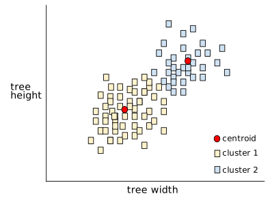
A human researcher could then review the clusters and, for example, label cluster 1 as "dwarf trees" and cluster 2 as "full-size trees."
As another example, consider a clustering algorithm based on an example's distance from a center point, illustrated as follows:
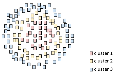
See the Clustering course for more information.
co-adaptation
An undesirable behavior in which neurons predict patterns in training data by relying almost exclusively on outputs of specific other neurons instead of relying on the network's behavior as a whole. When the patterns that cause co-adaptation are not present in validation data, then co-adaptation causes overfitting. Dropout regularization reduces co-adaptation because dropout ensures neurons cannot rely solely on specific other neurons.
collaborative filtering
Making predictions about the interests of one user based on the interests of many other users. Collaborative filtering is often used in recommendation systems.
See Collaborative filtering in the Recommendation Systems course for more information.
CommitmentBank (CB)
#Metric
A dataset for evaluating an LLM's proficiency in determining whether the author of a passage believes a target clause within that passage. Each entry in the dataset contains:
- A passage
- A target clause within that passage
- A Boolean value indicating whether the passage's author believes the target clause
For example:
- Passage: What fun to hear Artemis laugh. She's such a serious child. I didn't know she had a sense of humor.
- Target clause: she had a sense of humor
- Boolean: True, which means the author believes the target clause
CommitmentBank is a component of the SuperGLUE ensemble.
compact model
Any small model designed to run on small devices with limited computational resources. For example, compact models can run on mobile phones, tablets, or embedded systems.
compute
(Noun) The computational resources used by a model or system, such as processing power, memory, and storage.
See accelerator chips.
concept drift
A shift in the relationship between features and the label. Over time, concept drift reduces a model's quality.
During training, the model learns the relationship between the features and their labels in the training set. If the labels in the training set are good proxies for the real-world, then the model should make good real world predictions. However, due to concept drift, the model's predictions tend to degrade over time.
For example, consider a binary classification model that predicts whether or not a certain car model is "fuel efficient." That is, the features could be:
- car weight
- engine compression
- transmission type
while the label is either:
- fuel efficient
- not fuel efficient
However, the concept of "fuel efficient car" keeps changing. A car model labeled fuel efficient in 1994 would almost certainly be labeled not fuel efficient in 2024. A model suffering from concept drift tends to make less and less useful predictions over time.
Compare and contrast with nonstationarity.
Click the icon for additional notes.
To compensate for concept drift, retrain models faster than the rate of concept drift. For example, if concept drift reduces model precision by a meaningful margin every two months, then retrain your model more frequently than every two months.
condition
#df
In a decision tree, any node that performs a test. For example, the following decision tree contains two conditions:
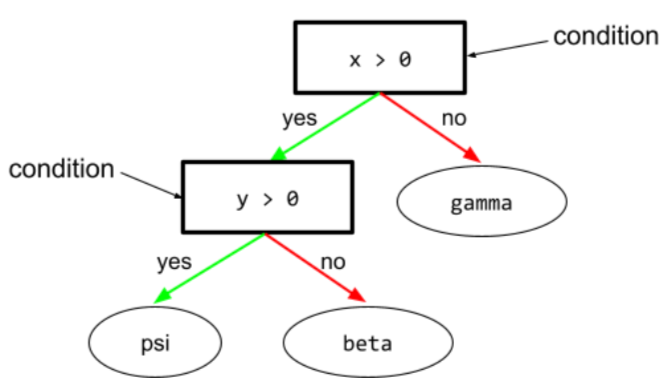
A condition is also called a split or a test.
Contrast condition with leaf.
See also:
See Types of conditions in the Decision Forests course for more information.
confabulation
Synonym for hallucination.
Confabulation is probably a more technically accurate term than hallucination. However, hallucination became popular first.
configuration
The process of assigning the initial property values used to train a model, including:
- the model's composing layers
- the location of the data
- hyperparameters such as:
In machine learning projects, configuration can be done through a special configuration file or using configuration libraries such as the following:
confirmation bias
#responsible
The tendency to search for, interpret, favor, and recall information in a way that confirms one's pre-existing beliefs or hypotheses. Machine learning developers may inadvertently collect or label data in ways that influence an outcome supporting their existing beliefs. Confirmation bias is a form of implicit bias.
Experimenter's bias is a form of confirmation bias in which an experimenter continues training models until a pre-existing hypothesis is confirmed.
confusion matrix
#fundamentals
An NxN table that summarizes the number of correct and incorrect predictions that a classification model made. For example, consider the following confusion matrix for a binary classification model:
| Tumor (predicted) | Non-Tumor (predicted) | |
|---|---|---|
| Tumor (ground truth) | 18 (TP) | 1 (FN) |
| Non-Tumor (ground truth) | 6 (FP) | 452 (TN) |
The preceding confusion matrix shows the following:
- Of the 19 predictions in which ground truth was Tumor, the model correctly classified 18 and incorrectly classified 1.
- Of the 458 predictions in which ground truth was Non-Tumor, the model correctly classified 452 and incorrectly classified 6.
The confusion matrix for a multi-class classification problem can help you identify patterns of mistakes. For example, consider the following confusion matrix for a 3-class multi-class classification model that categorizes three different iris types (Virginica, Versicolor, and Setosa). When the ground truth was Virginica, the confusion matrix shows that the model was far more likely to mistakenly predict Versicolor than Setosa:
| Setosa (predicted) | Versicolor (predicted) | Virginica (predicted) | |
|---|---|---|---|
| Setosa (ground truth) | 88 | 12 | 0 |
| Versicolor (ground truth) | 6 | 141 | 7 |
| Virginica (ground truth) | 2 | 27 | 109 |
As yet another example, a confusion matrix could reveal that a model trained to recognize handwritten digits tends to mistakenly predict 9 instead of 4, or mistakenly predict 1 instead of 7.
Confusion matrixes contain sufficient information to calculate a variety of performance metrics, including precision and recall.
constituency parsing
Dividing a sentence into smaller grammatical structures ("constituents"). A later part of the ML system, such as a natural language understanding model, can parse the constituents more easily than the original sentence. For example, consider the following sentence:
My friend adopted two cats.
A constituency parser can divide this sentence into the following two constituents:
- My friend is a noun phrase.
- adopted two cats is a verb phrase.
These constituents can be further subdivided into smaller constituents. For example, the verb phrase
adopted two cats
could be further subdivided into:
- adopted is a verb.
- two cats is another noun phrase.
contextualized language embedding
#generativeAI
An embedding that comes close to "understanding" words and phrases in ways that fluent human speakers can. Contextualized language embeddings can understand complex syntax, semantics, and context.
For example, consider embeddings of the English word cow. Older embeddings such as word2vec can represent English words such that the distance in the embedding space from cow to bull is similar to the distance from ewe (female sheep) to ram (male sheep) or from female to male. Contextualized language embeddings can go a step further by recognizing that English speakers sometimes casually use the word cow to mean either cow or bull.
context window
#generativeAI
The number of tokens a model can process in a given prompt. The larger the context window, the more information the model can use to provide coherent and consistent responses to the prompt.
continuous feature
#fundamentals
A floating-point feature with an infinite range of possible values, such as temperature or weight.
Contrast with discrete feature.
convenience sampling
Using a dataset not gathered scientifically in order to run quick experiments. Later on, it's essential to switch to a scientifically gathered dataset.
convergence
#fundamentals
A state reached when loss values change very little or not at all with each iteration. For example, the following loss curve suggests convergence at around 700 iterations:
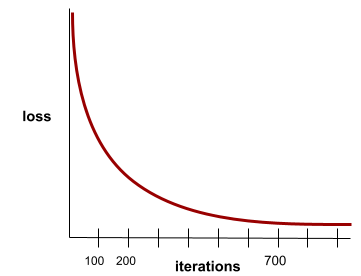
A model converges when additional training won't improve the model.
In deep learning, loss values sometimes stay constant or nearly so for many iterations before finally descending. During a long period of constant loss values, you may temporarily get a false sense of convergence.
See also early stopping.
See Model convergence and loss curves in Machine Learning Crash Course for more information.
conversational coding
#generativeAI
An iterative dialog between you and a generative AI model for the purpose of creating software. You issue a prompt describing some software. Then, the model uses that description to generate code. Then, you issue a new prompt to address the flaws in the previous prompt or in the generated code, and the model generates updated code. You two keep going back and forth until the generated software is good enough.
Conversation coding is essentially the original meaning of vibe coding.
Contrast with specificational coding.
convex function
A function in which the region above the graph of the function is a convex set. The prototypical convex function is shaped something like the letter U. For example, the following are all convex functions:
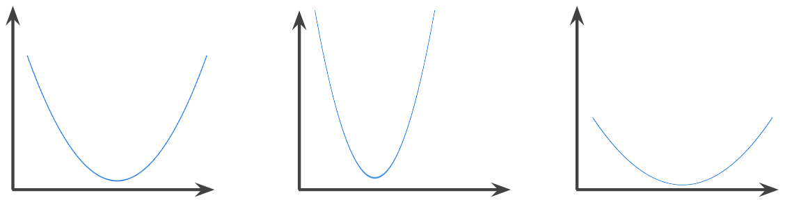
In contrast, the following function is not convex. Notice how the region above the graph is not a convex set:
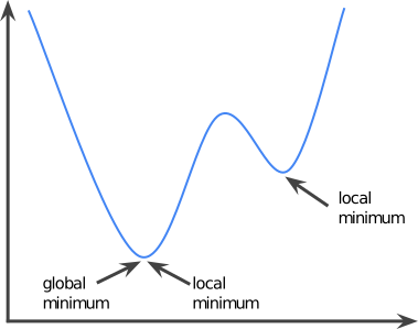
A strictly convex function has exactly one local minimum point, which is also the global minimum point. The classic U-shaped functions are strictly convex functions. However, some convex functions (for example, straight lines) are not U-shaped.
Click the icon for a deeper look at the math.
A lot of the common loss functions, including the following, are convex functions:
Many variations of gradient descent are guaranteed to find a point close to the minimum of a strictly convex function. Similarly, many variations of stochastic gradient descent have a high probability (though, not a guarantee) of finding a point close to the minimum of a strictly convex function.
The sum of two convex functions (for example, L2 loss + L1 regularization) is a convex function.
Deep models are never convex functions. Remarkably, algorithms designed for convex optimization tend to find reasonably good solutions on deep networks anyway, even though those solutions are not guaranteed to be a global minimum.
See Convergence and convex functions in Machine Learning Crash Course for more information.
convex optimization
The process of using mathematical techniques such as gradient descent to find the minimum of a convex function. A great deal of research in machine learning has focused on formulating various problems as convex optimization problems and in solving those problems more efficiently.
For complete details, see Boyd and Vandenberghe, Convex Optimization.
convex set
A subset of Euclidean space such that a line drawn between any two points in the subset remains completely within the subset. For instance, the following two shapes are convex sets:

In contrast, the following two shapes are not convex sets:

convolution
In mathematics, casually speaking, a mixture of two functions. In machine learning, a convolution mixes the convolutional filter and the input matrix in order to train weights.
The term "convolution" in machine learning is often a shorthand way of referring to either convolutional operation or convolutional layer.
Without convolutions, a machine learning algorithm would have to learn a separate weight for every cell in a large tensor. For example, a machine learning algorithm training on 2K x 2K images would be forced to find 4M separate weights. Thanks to convolutions, a machine learning algorithm only has to find weights for every cell in the convolutional filter, dramatically reducing the memory needed to train the model. When the convolutional filter is applied, it is simply replicated across cells such that each is multiplied by the filter.
convolutional filter
One of the two actors in a convolutional operation. (The other actor is a slice of an input matrix.) A convolutional filter is a matrix having the same rank as the input matrix, but a smaller shape. For example, given a 28x28 input matrix, the filter could be any 2D matrix smaller than 28x28.
In photographic manipulation, all the cells in a convolutional filter are typically set to a constant pattern of ones and zeroes. In machine learning, convolutional filters are typically seeded with random numbers and then the network trains the ideal values.
convolutional layer
A layer of a deep neural network in which a convolutional filter passes along an input matrix. For example, consider the following 3x3 convolutional filter:
![A 3x3 matrix with the following values: [[0,1,0], [1,0,1], [0,1,0]]](https://developers.google.com/static/machine-learning/glossary/images/ConvolutionalFilter33.svg)
The following animation shows a convolutional layer consisting of 9 convolutional operations involving the 5x5 input matrix. Notice that each convolutional operation works on a different 3x3 slice of the input matrix. The resulting 3x3 matrix (on the right) consists of the results of the 9 convolutional operations:
![An animation showing two matrixes. The first matrix is the 5x5
matrix: [[128,97,53,201,198], [35,22,25,200,195],
[37,24,28,197,182], [33,28,92,195,179], [31,40,100,192,177]].
The second matrix is the 3x3 matrix:
[[181,303,618], [115,338,605], [169,351,560]].
The second matrix is calculated by applying the convolutional
filter [[0, 1, 0], [1, 0, 1], [0, 1, 0]] across
different 3x3 subsets of the 5x5 matrix.](https://developers.google.com/static/machine-learning/glossary/images/AnimatedConvolution.gif)
convolutional neural network
A neural network in which at least one layer is a convolutional layer. A typical convolutional neural network consists of some combination of the following layers:
Convolutional neural networks have had great success in certain kinds of problems, such as image recognition.
convolutional operation
The following two-step mathematical operation:
- Element-wise multiplication of the convolutional filter and a slice of an input matrix. (The slice of the input matrix has the same rank and size as the convolutional filter.)
- Summation of all the values in the resulting product matrix.
For example, consider the following 5x5 input matrix:
![The 5x5 matrix: [[128,97,53,201,198], [35,22,25,200,195],
[37,24,28,197,182], [33,28,92,195,179], [31,40,100,192,177]].](https://developers.google.com/static/machine-learning/glossary/images/ConvolutionalLayerInputMatrix.svg)
Now imagine the following 2x2 convolutional filter:
![The 2x2 matrix: [[1, 0], [0, 1]]](https://developers.google.com/static/machine-learning/glossary/images/ConvolutionalLayerFilter.svg)
Each convolutional operation involves a single 2x2 slice of the input matrix. For example, suppose we use the 2x2 slice at the top-left of the input matrix. So, the convolution operation on this slice looks as follows:
![Applying the convolutional filter [[1, 0], [0, 1]] to the top-left
2x2 section of the input matrix, which is [[128,97], [35,22]].
The convolutional filter leaves the 128 and 22 intact, but zeroes
out the 97 and 35. Consequently, the convolution operation yields
the value 150 (128+22).](https://developers.google.com/static/machine-learning/glossary/images/ConvolutionalLayerOperation.svg)
A convolutional layer consists of a series of convolutional operations, each acting on a different slice of the input matrix.
COPA
#Metric
Abbreviation for Choice of Plausible Alternatives.
cost
#Metric
Synonym for loss.
co-training
A semi-supervised learning approach particularly useful when all of the following conditions are true:
- The ratio of unlabeled examples to labeled examples in the dataset is high.
- This is a classification problem (binary or multi-class).
- The dataset contains two different sets of predictive features that are independent of each other and complementary.
Co-training essentially amplifies independent signals into a stronger signal. For example, consider a classification model that categorizes individual used cars as either Good or Bad. One set of predictive features might focus on aggregate characteristics such as the year, make, and model of the car; another set of predictive features might focus on the previous owner's driving record and the car's maintenance history.
The seminal paper on co-training is Combining Labeled and Unlabeled Data with Co-Training by Blum and Mitchell.
counterfactual fairness
#responsible
#Metric
A fairness metric that checks whether a classification model produces the same result for one individual as it does for another individual who is identical to the first, except with respect to one or more sensitive attributes. Evaluating a classification model for counterfactual fairness is one method for surfacing potential sources of bias in a model.
See either of the following for more information:
- Fairness: Counterfactual fairness in Machine Learning Crash Course.
- When Worlds Collide: Integrating Different Counterfactual Assumptions in Fairness
coverage bias
#responsible
See selection bias.
crash blossom
A sentence or phrase with an ambiguous meaning. Crash blossoms present a significant problem in natural language understanding. For example, the headline Red Tape Holds Up Skyscraper is a crash blossom because an NLU model could interpret the headline literally or figuratively.
Click the icon for additional notes.
Just to clarify that mysterious headline:
- Red Tape could refer to either of the following:
- An adhesive
- Excessive bureaucracy
- Holds Up could refer to either of the following:
- Structural support
- Delays
critic
Synonym for Deep Q-Network.
cross-entropy
#Metric
A generalization of Log Loss to multi-class classification problems. Cross-entropy quantifies the difference between two probability distributions. See also perplexity.
cross-validation
A mechanism for estimating how well a model would generalize to new data by testing the model against one or more non-overlapping data subsets withheld from the training set.
cumulative distribution function (CDF)
#Metric
A function that defines the frequency of samples less than or equal to a target value. For example, consider a normal distribution of continuous values. A CDF tells you that approximately 50% of samples should be less than or equal to the mean and that approximately 84% of samples should be less than or equal to one standard deviation above the mean.
D
data analysis
Obtaining an understanding of data by considering samples, measurement, and visualization. Data analysis can be particularly useful when a dataset is first received, before one builds the first model. It is also crucial in understanding experiments and debugging problems with the system.
data augmentation
Artificially boosting the range and number of training examples by transforming existing examples to create additional examples. For example, suppose images are one of your features, but your dataset doesn't contain enough image examples for the model to learn useful associations. Ideally, you'd add enough labeled images to your dataset to enable your model to train properly. If that's not possible, data augmentation can rotate, stretch, and reflect each image to produce many variants of the original picture, possibly yielding enough labeled data to enable excellent training.
DataFrame
#fundamentals
A popular pandas data type for representing datasets in memory.
A DataFrame is analogous to a table or a spreadsheet. Each column of a DataFrame has a name (a header), and each row is identified by a unique number.
Each column in a DataFrame is structured like a 2D array, except that each column can be assigned its own data type.
See also the official pandas.DataFrame reference page.
data parallelism
A way of scaling training or inference that replicates an entire model onto multiple devices and then passes a subset of the input data to each device. Data parallelism can enable training and inference on very large batch sizes; however, data parallelism requires that the model be small enough to fit on all devices.
Data parallelism typically speeds training and inference.
See also model parallelism.
Dataset API (tf.data)
#TensorFlow
A high-level TensorFlow API for reading data and
transforming it into a form that a machine learning algorithm requires.
A tf.data.Dataset object represents a sequence of elements, in which
each element contains one or more Tensors. A tf.data.Iterator
object provides access to the elements of a Dataset.
data set or dataset
#fundamentals
A collection of raw data, commonly (but not exclusively) organized in one of the following formats:
- a spreadsheet
- a file in CSV (comma-separated values) format
decision boundary
The separator between classes learned by a model in a binary class or multi-class classification problems. For example, in the following image representing a binary classification problem, the decision boundary is the frontier between the orange class and the blue class:

decision forest
#df
A model created from multiple decision trees. A decision forest makes a prediction by aggregating the predictions of its decision trees. Popular types of decision forests include random forests and gradient boosted trees.
See the Decision Forests section in the Decision Forests course for more information.
decision threshold
Synonym for classification threshold.
decision tree
#df
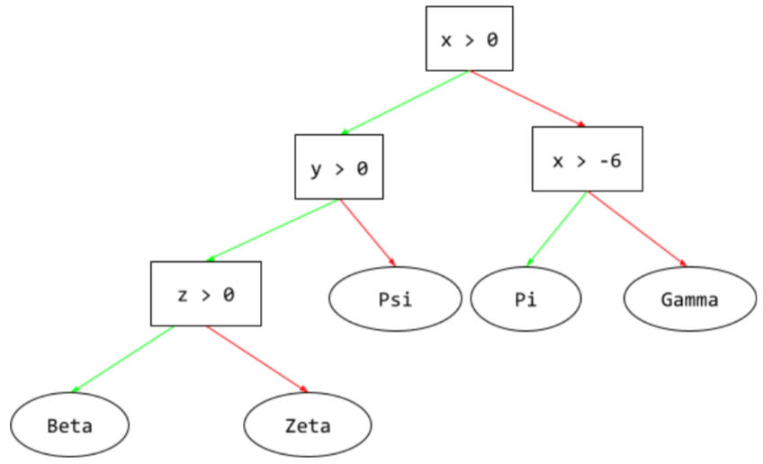
A supervised learning model composed of a set of conditions and leaves organized hierarchically. For example, the following is a decision tree:
decoder
In general, any ML system that converts from a processed, dense, or internal representation to a more raw, sparse, or external representation.
Decoders are often a component of a larger model, where they are frequently paired with an encoder.
In sequence-to-sequence tasks, a decoder starts with the internal state generated by the encoder to predict the next sequence.
Refer to Transformer for the definition of a decoder within the Transformer architecture.
See Large language models in Machine Learning Crash Course for more information.
deep model
#fundamentals
A neural network containing more than one hidden layer.
A deep model is also called a deep neural network.
Contrast with wide model.
deep neural network
Synonym for deep model.
Deep Q-Network (DQN)
In Q-learning, a deep neural network that predicts Q-functions.
Critic is a synonym for Deep Q-Network.
demographic parity
#responsible
#Metric
A fairness metric that is satisfied if the results of a model's classification are not dependent on a given sensitive attribute.
For example, if both Lilliputians and Brobdingnagians apply to Glubbdubdrib University, demographic parity is achieved if the percentage of Lilliputians admitted is the same as the percentage of Brobdingnagians admitted, irrespective of whether one group is on average more qualified than the other.
Contrast with equalized odds and equality of opportunity, which permit classification results in aggregate to depend on sensitive attributes, but don't permit classification results for certain specified ground truth labels to depend on sensitive attributes. See "Attacking discrimination with smarter machine learning" for a visualization exploring the tradeoffs when optimizing for demographic parity.
See Fairness: demographic parity in Machine Learning Crash Course for more information.
denoising
A common approach to self-supervised learning in which:
Denoising enables learning from unlabeled examples. The original dataset serves as the target or label and the noisy data as the input.
Some masked language models use denoising as follows:
- Noise is artificially added to an unlabeled sentence by masking some of the tokens.
- The model tries to predict the original tokens.
dense feature
#fundamentals
A feature in which most or all values are nonzero, typically a Tensor of floating-point values. For example, the following 10-element Tensor is dense because 9 of its values are nonzero:
| 8 | 3 | 7 | 5 | 2 | 4 | 0 | 4 | 9 | 6 |
Contrast with sparse feature.
dense layer
Synonym for fully connected layer.
depth
#fundamentals
The sum of the following in a neural network:
- the number of hidden layers
- the number of output layers, which is typically 1
- the number of any embedding layers
For example, a neural network with five hidden layers and one output layer has a depth of 6.
Notice that the input layer doesn't influence depth.
depthwise separable convolutional neural network (sepCNN)
A convolutional neural network architecture based on Inception, but where Inception modules are replaced with depthwise separable convolutions. Also known as Xception.
A depthwise separable convolution (also abbreviated as separable convolution) factors a standard 3D convolution into two separate convolution operations that are more computationally efficient: first, a depthwise convolution, with a depth of 1 (n ✕ n ✕ 1), and then second, a pointwise convolution, with length and width of 1 (1 ✕ 1 ✕ n).
To learn more, see Xception: Deep Learning with Depthwise Separable Convolutions.
derived label
Synonym for proxy label.
deterministic
A system that always returns the same output for a given input. For example, the ReLU function is deterministic because:
- When the input is negative, the output is always 0.
- When the input is nonnegative, the output always equals the input.
By contrast, a function that returns a random number each time it is called is nondeterministic.
Deterministic systems are generally much easier to test than nondeterministic systems.
LLMs are usually nondeterministic; that is, the LLM's response to the same prompt often differs.
device
#TensorFlow
#GoogleCloud
An overloaded term with the following two possible definitions:
- A category of hardware that can run a TensorFlow session, including CPUs, GPUs, and TPUs.
- When training an ML model on accelerator chips (GPUs or TPUs), the part of the system that actually manipulates tensors and embeddings. The device runs on accelerator chips. In contrast, the host typically runs on a CPU.
differential privacy
In machine learning, an anonymization approach to protect any sensitive data (for example, an individual's personal information) included in a model's training set from being exposed. This approach ensures that the model doesn't learn or remember much about a specific individual. This is accomplished by sampling and adding noise during model training to obscure individual data points, mitigating the risk of exposing sensitive training data.
Differential privacy is also used outside of machine learning. For example, data scientists sometimes use differential privacy to protect individual privacy when computing product usage statistics for different demographics.
dimension reduction
Decreasing the number of dimensions used to represent a particular feature in a feature vector, typically by converting to an embedding vector.
dimensions
Overloaded term having any of the following definitions:
The number of levels of coordinates in a Tensor. For example:
- A scalar has zero dimensions; for example,
["Hello"]. - A vector has one dimension; for example,
[3, 5, 7, 11]. - A matrix has two dimensions; for example,
[[2, 4, 18], [5, 7, 14]]. You can uniquely specify a particular cell in a one-dimensional vector with one coordinate; you need two coordinates to uniquely specify a particular cell in a two-dimensional matrix.
- A scalar has zero dimensions; for example,
The number of entries in a feature vector.
The number of elements in an embedding layer.
direct prompting
#generativeAI
Synonym for zero-shot prompting.
discrete feature
#fundamentals
A feature with a finite set of possible values. For example, a feature whose values may only be animal, vegetable, or mineral is a discrete (or categorical) feature.
Contrast with continuous feature.
discriminative model
A model that predicts labels from a set of one or more features. More formally, discriminative models define the conditional probability of an output given the features and weights; that is:
p(output | features, weights)
For example, a model that predicts whether an email is spam from features and weights is a discriminative model.
The vast majority of supervised learning models, including classification and regression models, are discriminative models.
Contrast with generative model.
discriminator
A system that determines whether examples are real or fake.
Alternatively, the subsystem within a generative adversarial network that determines whether the examples created by the generator are real or fake.
See The discriminator in the GAN course for more information.
disparate impact
#responsible
Making decisions about people that impact different population subgroups disproportionately. This usually refers to situations where an algorithmic decision-making process harms or benefits some subgroups more than others.
For example, suppose an algorithm that determines a Lilliputian's eligibility for a miniature-home loan is more likely to classify them as "ineligible" if their mailing address contains a certain postal code. If Big-Endian Lilliputians are more likely to have mailing addresses with this postal code than Little-Endian Lilliputians, then this algorithm may result in disparate impact.
Contrast with disparate treatment, which focuses on disparities that result when subgroup characteristics are explicit inputs to an algorithmic decision-making process.
disparate treatment
#responsible
Factoring subjects' sensitive attributes into an algorithmic decision-making process such that different subgroups of people are treated differently.
For example, consider an algorithm that determines Lilliputians' eligibility for a miniature-home loan based on the data they provide in their loan application. If the algorithm uses a Lilliputian's affiliation as Big-Endian or Little-Endian as an input, it is enacting disparate treatment along that dimension.
Contrast with disparate impact, which focuses on disparities in the societal impacts of algorithmic decisions on subgroups, irrespective of whether those subgroups are inputs to the model.
distillation
#generativeAI
The process of reducing the size of one model (known as the teacher) into a smaller model (known as the student) that emulates the original model's predictions as faithfully as possible. Distillation is useful because the smaller model has two key benefits over the larger model (the teacher):
- Faster inference time
- Reduced memory and energy usage
However, the student's predictions are typically not as good as the teacher's predictions.
Distillation trains the student model to minimize a loss function based on the difference between the outputs of the predictions of the student and teacher models.
Compare and contrast distillation with the following terms:
See LLMs: Fine-tuning, distillation, and prompt engineering in Machine Learning Crash Course for more information.
distribution
The frequency and range of different values for a given feature or label. A distribution captures how likely a particular value is.
The following image shows histograms of two different distributions:
- On the left, a power law distribution of wealth versus the number of people possessing that wealth.
- On the right, a normal distribution of height versus the number of people possessing that height.
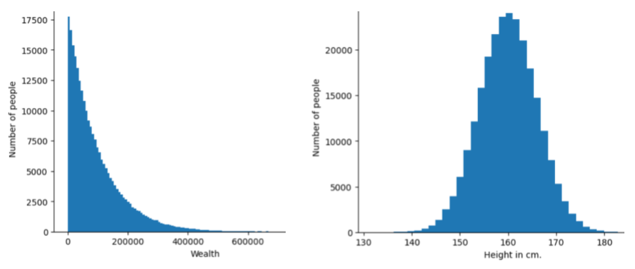
Understanding each feature and label's distribution can help you determine how to normalize values and detect outliers.
The phrase out of distribution refers to a value that doesn't appear in the dataset or is very rare. For example, an image of the planet Saturn would be considered out of distribution for a dataset consisting of cat images.
divisive clustering
#clustering
downsampling
Overloaded term that can mean either of the following:
- Reducing the amount of information in a feature in order to train a model more efficiently. For example, before training an image recognition model, downsampling high-resolution images to a lower-resolution format.
- Training on a disproportionately low percentage of over-represented class examples in order to improve model training on under-represented classes. For example, in a class-imbalanced dataset, models tend to learn a lot about the majority class and not enough about the minority class. Downsampling helps balance the amount of training on the majority and minority classes.
See Datasets: Imbalanced datasets in Machine Learning Crash Course for more information.
DQN
Abbreviation for Deep Q-Network.
dropout regularization
A form of regularization useful in training neural networks. Dropout regularization removes a random selection of a fixed number of the units in a network layer for a single gradient step. The more units dropped out, the stronger the regularization. This is analogous to training the network to emulate an exponentially large ensemble of smaller networks. For full details, see Dropout: A Simple Way to Prevent Neural Networks from Overfitting.
dynamic
#fundamentals
Something done frequently or continuously. The terms dynamic and online are synonyms in machine learning. The following are common uses of dynamic and online in machine learning:
- A dynamic model (or online model) is a model that is retrained frequently or continuously.
- Dynamic training (or online training) is the process of training frequently or continuously.
- Dynamic inference (or online inference) is the process of generating predictions on demand.
dynamic model
#fundamentals
A model that is frequently (maybe even continuously) retrained. A dynamic model is a "lifelong learner" that constantly adapts to evolving data. A dynamic model is also known as an online model.
Contrast with static model.
E
eager execution
#TensorFlow
A TensorFlow programming environment in which operations run immediately. In contrast, operations called in graph execution don't run until they are explicitly evaluated. Eager execution is an imperative interface, much like the code in most programming languages. Eager execution programs are generally far easier to debug than graph execution programs.
early stopping
#fundamentals
A method for regularization that involves ending training before training loss finishes decreasing. In early stopping, you intentionally stop training the model when the loss on a validation dataset starts to increase; that is, when generalization performance worsens.
Click the icon for additional notes.
Early stopping may seem counterintuitive. After all, telling a model to halt training while the loss is still decreasing may seem like telling a chef to stop cooking before the dessert has fully baked. However, training a model for too long can lead to overfitting. That is, if you train a model too long, the model may fit the training data so closely that the model doesn't make good predictions on new examples.
Contrast with early exit.
earth mover's distance (EMD)
#Metric
A measure of the relative similarity of two distributions. The lower the earth mover's distance, the more similar the distributions.
edit distance
#Metric
A measurement of how similar two text strings are to each other. In machine learning, edit distance is useful for the following reasons:
- Edit distance is easy to compute.
- Edit distance can compare two strings known to be similar to each other.
- Edit distance can determine the degree to which different strings are similar to a given string.
Several definitions of edit distance exist, each using different string operations. See Levenshtein distance for an example.
Einsum notation
An efficient notation for describing how two tensors are to be combined. The tensors are combined by multiplying the elements of one tensor by the elements of the other tensor and then summing the products. Einsum notation uses symbols to identify the axes of each tensor, and those same symbols are rearranged to specify the shape of the new resulting tensor.
NumPy provides a common Einsum implementation.
embedding layer
#fundamentals
A special hidden layer that trains on a high-dimensional categorical feature to gradually learn a lower dimension embedding vector. An embedding layer enables a neural network to train far more efficiently than training just on the high-dimensional categorical feature.
For example, Earth currently supports about 73,000 tree species. Suppose
tree species is a feature in your model, so your model's
input layer includes a one-hot vector 73,000
elements long.
For example, perhaps baobab would be represented something like this:

A 73,000-element array is very long. If you don't add an embedding layer to the model, training is going to be very time consuming due to multiplying 72,999 zeros. Perhaps you pick the embedding layer to consist of 12 dimensions. Consequently, the embedding layer will gradually learn a new embedding vector for each tree species.
In certain situations, hashing is a reasonable alternative to an embedding layer.
See Embeddings in Machine Learning Crash Course for more information.
embedding space
The d-dimensional vector space that features from a higher-dimensional vector space are mapped to. Embedding space is trained to capture structure that is meaningful for the intended application.
The dot product of two embeddings is a measure of their similarity.
embedding vector
Broadly speaking, an array of floating-point numbers taken from any hidden layer that describe the inputs to that hidden layer. Often, an embedding vector is the array of floating-point numbers trained in an embedding layer. For example, suppose an embedding layer must learn an embedding vector for each of the 73,000 tree species on Earth. Perhaps the following array is the embedding vector for a baobab tree:

An embedding vector is not a bunch of random numbers. An embedding layer determines these values through training, similar to the way a neural network learns other weights during training. Each element of the array is a rating along some characteristic of a tree species. Which element represents which tree species' characteristic? That's very hard for humans to determine.
The mathematically remarkable part of an embedding vector is that similar items have similar sets of floating-point numbers. For example, similar tree species have a more similar set of floating-point numbers than dissimilar tree species. Redwoods and sequoias are related tree species, so they'll have a more similar set of floating-pointing numbers than redwoods and coconut palms. The numbers in the embedding vector will change each time you retrain the model, even if you retrain the model with identical input.
emergent behavior
An LLM's ability to generate responses for prompts that it was not explicitly trained on.
empirical cumulative distribution function (eCDF or EDF)
#Metric
A cumulative distribution function based on empirical measurements from a real dataset. The value of the function at any point along the x-axis is the fraction of observations in the dataset that are less than or equal to the specified value.
empirical risk minimization (ERM)
Choosing the function that minimizes loss on the training set. Contrast with structural risk minimization.
encoder
In general, any ML system that converts from a raw, sparse, or external representation into a more processed, denser, or more internal representation.
Encoders are often a component of a larger model, where they are frequently paired with a decoder. Some Transformers pair encoders with decoders, though other Transformers use only the encoder or only the decoder.
Some systems use the encoder's output as the input to a classification or regression network.
In sequence-to-sequence tasks, an encoder takes an input sequence and returns an internal state (a vector). Then, the decoder uses that internal state to predict the next sequence.
Refer to Transformer for the definition of an encoder in the Transformer architecture.
See LLMs: What's a large language model in Machine Learning Crash Course for more information.
endpoints
A network-addressable location (typically a URL) where a service can be reached.
ensemble
A collection of models trained independently whose predictions are averaged or aggregated. In many cases, an ensemble produces better predictions than a single model. For example, a random forest is an ensemble built from multiple decision trees. Note that not all decision forests are ensembles.
See Random Forest in Machine Learning Crash Course for more information.
entropy
#df
#Metric
In information theory, a description of how unpredictable a probability distribution is. Alternatively, entropy is also defined as how much information each example contains. A distribution has the highest possible entropy when all values of a random variable are equally likely.
The entropy of a set with two possible values "0" and "1" (for example, the labels in a binary classification problem) has the following formula:
H = -p log p - q log q = -p log p - (1-p) * log (1-p)
where:
- H is the entropy.
- p is the fraction of "1" examples.
- q is the fraction of "0" examples. Note that q = (1 - p)
- log is generally log2. In this case, the entropy unit is a bit.
For example, suppose the following:
- 100 examples contain the value "1"
- 300 examples contain the value "0"
Therefore, the entropy value is:
- p = 0.25
- q = 0.75
- H = (-0.25)log2(0.25) - (0.75)log2(0.75) = 0.81 bits per example
A set that is perfectly balanced (for example, 200 "0"s and 200 "1"s) would have an entropy of 1.0 bit per example. As a set becomes more imbalanced, its entropy moves towards 0.0.
In decision trees, entropy helps formulate information gain to help the splitter select the conditions during the growth of a classification decision tree.
Compare entropy with:
- gini impurity
- cross-entropy loss function
Entropy is often called Shannon's entropy.
See Exact splitter for binary classification with numerical features in the Decision Forests course for more information.
environment
In reinforcement learning, the world that contains the agent and allows the agent to observe that world's state. For example, the represented world can be a game like chess, or a physical world like a maze. When the agent applies an action to the environment, then the environment transitions between states.
environment grounding
The raw data that flows back to the agent during the feedback stage of the agentic loop. For example, environment grounding for an agent might include error logs or the HTML of a newly created web page.
episode
In reinforcement learning, each of the repeated attempts by the agent to learn an environment.
episodic memory
In LLMs, information learned after training. In contrast, semantic memory is information learned during training. Episodic memory can be temporary (for example, lasting only within the current chatbot session) or more permanent (for example, persisting for each session the user invokes).
See also procedural memory.
epoch
#fundamentals
A full training pass over the entire training set such that each example has been processed once.
An epoch represents N/batch size
training iterations, where N is the
total number of examples.
For instance, suppose the following:
- The dataset consists of 1,000 examples.
- The batch size is 50 examples.
Therefore, a single epoch requires 20 iterations:
1 epoch = (N/batch size) = (1,000 / 50) = 20 iterations
See Linear regression: Hyperparameters in Machine Learning Crash Course for more information.
epsilon greedy policy
In reinforcement learning, a policy that either follows a random policy with epsilon probability or a greedy policy otherwise. For example, if epsilon is 0.9, then the policy follows a random policy 90% of the time and a greedy policy 10% of the time.
Over successive episodes, the algorithm reduces epsilon's value in order to shift from following a random policy to following a greedy policy. By shifting the policy, the agent first randomly explores the environment and then greedily exploits the results of random exploration.
equality of opportunity
#responsible
#Metric
A fairness metric to assess whether a model is predicting the desirable outcome equally well for all values of a sensitive attribute. In other words, if the desirable outcome for a model is the positive class, the goal would be to have the true positive rate be the same for all groups.
Equality of opportunity is related to equalized odds, which requires that both the true positive rates and false positive rates are the same for all groups.
Suppose Glubbdubdrib University admits both Lilliputians and Brobdingnagians to a rigorous mathematics program. Lilliputians' secondary schools offer a robust curriculum of math classes, and the vast majority of students are qualified for the university program. Brobdingnagians' secondary schools don't offer math classes at all, and as a result, far fewer of their students are qualified. Equality of opportunity is satisfied for the preferred label of "admitted" with respect to nationality (Lilliputian or Brobdingnagian) if qualified students are equally likely to be admitted irrespective of whether they're a Lilliputian or a Brobdingnagian.
For example, suppose 100 Lilliputians and 100 Brobdingnagians apply to Glubbdubdrib University, and admissions decisions are made as follows:
Table 1. Lilliputian applicants (90% are qualified)
| Qualified | Unqualified | |
|---|---|---|
| Admitted | 45 | 3 |
| Rejected | 45 | 7 |
| Total | 90 | 10 |
|
Percentage of qualified students admitted: 45/90 = 50% Percentage of unqualified students rejected: 7/10 = 70% Total percentage of Lilliputian students admitted: (45+3)/100 = 48% |
||
Table 2. Brobdingnagian applicants (10% are qualified):
| Qualified | Unqualified | |
|---|---|---|
| Admitted | 5 | 9 |
| Rejected | 5 | 81 |
| Total | 10 | 90 |
|
Percentage of qualified students admitted: 5/10 = 50% Percentage of unqualified students rejected: 81/90 = 90% Total percentage of Brobdingnagian students admitted: (5+9)/100 = 14% |
||
The preceding examples satisfy equality of opportunity for acceptance of qualified students because qualified Lilliputians and Brobdingnagians both have a 50% chance of being admitted.
While equality of opportunity is satisfied, the following two fairness metrics are not satisfied:
- demographic parity: Lilliputians and Brobdingnagians are admitted to the university at different rates; 48% of Lilliputians students are admitted, but only 14% of Brobdingnagian students are admitted.
- equalized odds: While qualified Lilliputian and Brobdingnagian students both have the same chance of being admitted, the additional constraint that unqualified Lilliputians and Brobdingnagians both have the same chance of being rejected is not satisfied. Unqualified Lilliputians have a 70% rejection rate, whereas unqualified Brobdingnagians have a 90% rejection rate.
See Fairness: Equality of opportunity in Machine Learning Crash Course for more information.
equalized odds
#responsible
#Metric
A fairness metric to assess whether a model is predicting outcomes equally well for all values of a sensitive attribute with respect to both the positive class and negative class—not just one class or the other exclusively. In other words, both the true positive rate and false negative rate should be the same for all groups.
Equalized odds is related to equality of opportunity, which only focuses on error rates for a single class (positive or negative).
For example, suppose Glubbdubdrib University admits both Lilliputians and Brobdingnagians to a rigorous mathematics program. Lilliputians' secondary schools offer a robust curriculum of math classes, and the vast majority of students are qualified for the university program. Brobdingnagians' secondary schools don't offer math classes at all, and as a result, far fewer of their students are qualified. Equalized odds is satisfied provided that no matter whether an applicant is a Lilliputian or a Brobdingnagian, if they are qualified, they are equally as likely to get admitted to the program, and if they are not qualified, they are equally as likely to get rejected.
Suppose 100 Lilliputians and 100 Brobdingnagians apply to Glubbdubdrib University, and admissions decisions are made as follows:
Table 3. Lilliputian applicants (90% are qualified)
| Qualified | Unqualified | |
|---|---|---|
| Admitted | 45 | 2 |
| Rejected | 45 | 8 |
| Total | 90 | 10 |
|
Percentage of qualified students admitted: 45/90 = 50% Percentage of unqualified students rejected: 8/10 = 80% Total percentage of Lilliputian students admitted: (45+2)/100 = 47% |
||
Table 4. Brobdingnagian applicants (10% are qualified):
| Qualified | Unqualified | |
|---|---|---|
| Admitted | 5 | 18 |
| Rejected | 5 | 72 |
| Total | 10 | 90 |
|
Percentage of qualified students admitted: 5/10 = 50% Percentage of unqualified students rejected: 72/90 = 80% Total percentage of Brobdingnagian students admitted: (5+18)/100 = 23% |
||
Equalized odds is satisfied because qualified Lilliputian and Brobdingnagian students both have a 50% chance of being admitted, and unqualified Lilliputian and Brobdingnagian have an 80% chance of being rejected.
Equalized odds is formally defined in "Equality of Opportunity in Supervised Learning" as follows: "predictor Ŷ satisfies equalized odds with respect to protected attribute A and outcome Y if Ŷ and A are independent, conditional on Y."
Estimator
#TensorFlow
A deprecated TensorFlow API. Use tf.keras instead of Estimators.
evals
#generativeAI
#Metric
Primarily used as an abbreviation for LLM evaluations. More broadly, evals is an abbreviation for any form of evaluation.
evaluation
#generativeAI
#Metric
The process of measuring a model's quality or comparing different models against each other.
To evaluate a supervised machine learning model, you typically judge it against a validation set and a test set. Evaluating a LLM typically involves broader quality and safety assessments.
evaluator agent
#agent
An agent that assesses another agent's results before those results are finalized. You can imagine one agent as manufacturing a product and a separate agent—the evaluator agent—testing that product before it is released.
Critic is a synonym for evaluator agent.
exact match
#Metric
An all-or-nothing metric in which the model's output either matches ground truth or the reference text exactly or it doesn't. For example, if ground truth is orange, the only model output that satisfies exact match is orange.
Exact match can also evaluate models whose output is a sequence (a ranked list of items). In general, exact match requires the generated ranked list to exactly match ground truth; that is, each item in both lists must be in the same order. That said, if ground truth consists of multiple correct sequences, then exact match only requires model's output matches one of the correct sequences.
example
#fundamentals
The values of one row of features and possibly a label. Examples in supervised learning fall into two general categories:
- A labeled example consists of one or more features and a label. Labeled examples are used during training.
- An unlabeled example consists of one or more features but no label. Unlabeled examples are used during inference.
For instance, suppose you are training a model to determine the influence of weather conditions on student test scores. Here are three labeled examples:
| Features | Label | ||
|---|---|---|---|
| Temperature | Humidity | Pressure | Test score |
| 15 | 47 | 998 | Good |
| 19 | 34 | 1020 | Excellent |
| 18 | 92 | 1012 | Poor |
Here are three unlabeled examples:
| Temperature | Humidity | Pressure | |
|---|---|---|---|
| 12 | 62 | 1014 | |
| 21 | 47 | 1017 | |
| 19 | 41 | 1021 |
The row of a dataset is typically the raw source for an example. That is, an example typically consists of a subset of the columns in the dataset. Furthermore, the features in an example can also include synthetic features, such as feature crosses.
See Supervised Learning in the Introduction to Machine Learning course for more information.
experience replay
In reinforcement learning, a DQN technique used to reduce temporal correlations in training data. The agent stores state transitions in a replay buffer, and then samples transitions from the replay buffer to create training data.
experimenter's bias
#responsible
See confirmation bias.
exploding gradient problem
The tendency for gradients in deep neural networks (especially recurrent neural networks) to become surprisingly steep (high). Steep gradients often cause very large updates to the weights of each node in a deep neural network.
Models suffering from the exploding gradient problem become difficult or impossible to train. Gradient clipping can mitigate this problem.
Compare to vanishing gradient problem.
Extreme Summarization (xsum)
#Metric
A dataset for evaluating an LLM's ability to summarize a single document. Each entry in the dataset consists of:
- A document authored by the British Broadcasting Corporation (BBC).
- A one-sentence summary of that document.
For details, see Don't Give Me the Details, Just the Summary! Topic-Aware Convolutional Neural Networks for Extreme Summarization.
F
F1
#Metric
A "roll-up" binary classification metric that relies on both precision and recall. Here is the formula:
$$F{_1} = \frac{\text{2 * precision * recall}} {\text{precision + recall}}$$
Click the icon to see examples.
Suppose precision and recall have the following values:
- precision = 0.6
- recall = 0.4
You calculate F1 as follows:
$$F{_1} = \frac{\text{2 * 0.6 * 0.4}} {\text{0.6 + 0.4}} = 0.48$$
When precision and recall are fairly similar (as in the preceding example), F1 is close to their mean. When precision and recall differ significantly, F1 is closer to the lower value. For example:
- precision = 0.9
- recall = 0.1
$$F{_1} = \frac{\text{2 * 0.9 * 0.1}} {\text{0.9 + 0.1}} = 0.18$$
factuality
#generativeAI
Within the ML world, a property describing a model whose output is based on reality. Factuality is a concept rather than a metric. For example, suppose you send the following prompt to a large language model:
What is the chemical formula for table salt?
A model optimizing factuality would respond:
NaCl
It is tempting to assume that all models should be based on factuality. However, some prompts, such as the following, should cause a generative AI model to optimize creativity rather than factuality.
Tell me a limerick about an astronaut and a caterpillar.
It is unlikely that the resulting limerick would be based on reality.
Contrast with groundedness.
fairness constraint
#responsible
Applying a constraint to an algorithm to ensure one or more definitions of fairness are satisfied. Examples of fairness constraints include:
- Post-processing your model's output.
- Altering the loss function to incorporate a penalty for violating a fairness metric.
- Directly adding a mathematical constraint to an optimization problem.
fairness metric
#responsible
#Metric
A mathematical definition of "fairness" that is measurable. Some commonly used fairness metrics include:
Many fairness metrics are mutually exclusive; see incompatibility of fairness metrics.
false negative (FN)
#fundamentals
#Metric
An example in which the model mistakenly predicts the negative class. For example, the model predicts that a particular email message is not spam (the negative class), but that email message actually is spam.
false negative rate
#Metric
The proportion of actual positive examples for which the model mistakenly predicted the negative class. The following formula calculates the false negative rate:
$$\text{false negative rate} = \frac{\text{false negatives}}{\text{false negatives} + \text{true positives}}$$
See Thresholds and the confusion matrix in Machine Learning Crash Course for more information.
false positive (FP)
#fundamentals
#Metric
An example in which the model mistakenly predicts the positive class. For example, the model predicts that a particular email message is spam (the positive class), but that email message is actually not spam.
See Thresholds and the confusion matrix in Machine Learning Crash Course for more information.
false positive rate (FPR)
#fundamentals
#Metric
The proportion of actual negative examples for which the model mistakenly predicted the positive class. The following formula calculates the false positive rate:
$$\text{false positive rate} = \frac{\text{false positives}}{\text{false positives} + \text{true negatives}}$$
The false positive rate is the x-axis in an ROC curve.
See Classification: ROC and AUC in Machine Learning Crash Course for more information.
fast decay
#generativeAI
A training technique to improve the performance of LLMs. Fast decay involves rapidly decreasing the learning rate during training. This strategy helps prevent the model from overfitting to the training data, and improves generalization.
feature
#fundamentals
An input variable to a machine learning model. An example consists of one or more features. For instance, suppose you are training a model to determine the influence of weather conditions on student test scores. The following table shows three examples, each of which contains three features and one label:
| Features | Label | ||
|---|---|---|---|
| Temperature | Humidity | Pressure | Test score |
| 15 | 47 | 998 | 92 |
| 19 | 34 | 1020 | 84 |
| 18 | 92 | 1012 | 87 |
Contrast with label.
See Supervised Learning in the Introduction to Machine Learning course for more information.
feature cross
#fundamentals
A synthetic feature formed by "crossing" categorical or bucketed features.
For example, consider a "mood forecasting" model that represents temperature in one of the following four buckets:
freezingchillytemperatewarm
And represents wind speed in one of the following three buckets:
stilllightwindy
Without feature crosses, the linear model trains independently on each of the
preceding seven various buckets. So, the model trains on, for example,
freezing independently of the training on, for example,
windy.
Alternatively, you could create a feature cross of temperature and wind speed. This synthetic feature would have the following 12 possible values:
freezing-stillfreezing-lightfreezing-windychilly-stillchilly-lightchilly-windytemperate-stilltemperate-lighttemperate-windywarm-stillwarm-lightwarm-windy
Thanks to feature crosses, the model can learn mood differences
between a freezing-windy day and a freezing-still day.
If you create a synthetic feature from two features that each have a lot of different buckets, the resulting feature cross will have a huge number of possible combinations. For example, if one feature has 1,000 buckets and the other feature has 2,000 buckets, the resulting feature cross has 2,000,000 buckets.
Formally, a cross is a Cartesian product.
Feature crosses are mostly used with linear models and are rarely used with neural networks.
See Categorical data: Feature crosses in Machine Learning Crash Course for more information.
feature engineering
#fundamentals
#TensorFlow
A process that involves the following steps:
- Determining which features might be useful in training a model.
- Converting raw data from the dataset into efficient versions of those features.
For example, you might determine that temperature might be a useful
feature. Then, you might experiment with bucketing
to optimize what the model can learn from different temperature ranges.
Feature engineering is sometimes called feature extraction or featurization.
Click the icon for additional notes about TensorFlow.
In TensorFlow, feature engineering often means converting raw log file entries to tf.Example protocol buffers. See also tf.Transform.
See Numerical data: How a model ingests data using feature vectors in Machine Learning Crash Course for more information.
Overloaded term having either of the following definitions:
- Retrieving intermediate feature representations calculated by an unsupervised or pre-trained model (for example, hidden layer values in a neural network) for use in another model as input.
- Synonym for feature engineering.
feature importances
#df
#Metric
Synonym for variable importances.
feature set
#fundamentals
The group of features your machine learning model trains on. For example, a simple feature set for a model that predicts housing prices might consist of postal code, property size, and property condition.
feature spec
#TensorFlow
Describes the information required to extract features data from the tf.Example protocol buffer. Because the tf.Example protocol buffer is just a container for data, you must specify the following:
- The data to extract (that is, the keys for the features)
- The data type (for example, float or int)
- The length (fixed or variable)
feature vector
#fundamentals
The array of feature values comprising an example. The feature vector is input during training and during inference. For example, the feature vector for a model with two discrete features might be:
[0.92, 0.56]
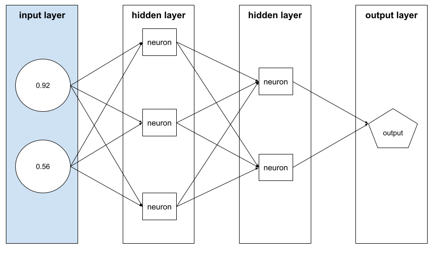
Each example supplies different values for the feature vector, so the feature vector for the next example could be something like:
[0.73, 0.49]
Feature engineering determines how to represent features in the feature vector. For example, a binary categorical feature with five possible values might be represented with one-hot encoding. In this case, the portion of the feature vector for a particular example would consist of four zeroes and a single 1.0 in the third position, as follows:
[0.0, 0.0, 1.0, 0.0, 0.0]
As another example, suppose your model consists of three features:
- a binary categorical feature with five possible values represented with
one-hot encoding; for example:
[0.0, 1.0, 0.0, 0.0, 0.0] - another binary categorical feature with three possible values represented
with one-hot encoding; for example:
[0.0, 0.0, 1.0] - a floating-point feature; for example:
8.3.
In this case, the feature vector for each example would be represented by nine values. Given the example values in the preceding list, the feature vector would be:
0.0
1.0
0.0
0.0
0.0
0.0
0.0
1.0
8.3
See Numerical data: How a model ingests data using feature vectors in Machine Learning Crash Course for more information.
featurization
The process of extracting features from an input source, such as a document or video, and mapping those features into a feature vector.
Some ML experts use featurization as a synonym for feature engineering or feature extraction.
federated learning
A distributed machine learning approach that trains machine learning models using decentralized examples residing on devices such as smartphones. In federated learning, a subset of devices downloads the current model from a central coordinating server. The devices use the examples stored on the devices to make improvements to the model. The devices then upload the model improvements (but not the training examples) to the coordinating server, where they are aggregated with other updates to yield an improved global model. After the aggregation, the model updates computed by devices are no longer needed, and can be discarded.
Since the training examples are never uploaded, federated learning follows the privacy principles of focused data collection and data minimization.
See the Federated Learning comic (yes, a comic) for more details.
feedback
#agent
A stage in an agentic loop in which the agent evaluates the action taken during the act stage. For example, if the agent sent an API request during the act stage, the feedback stage might determine whether the API response was successful.
feedback loop
#fundamentals
In machine learning, a situation in which a model's predictions influence the training data for the same model or another model. For example, a model that recommends movies will influence the movies that people see, which will then influence subsequent movie recommendation models.
See Production ML systems: Questions to ask in Machine Learning Crash Course for more information.
feedforward neural network (FFN)
A neural network without cyclic or recursive connections. For example, traditional deep neural networks are feedforward neural networks. Contrast with recurrent neural networks, which are cyclic.
few-shot learning
A machine learning approach, often used for object classification, designed to train effective classification models from only a small number of training examples.
See also one-shot learning and zero-shot learning.
few-shot prompting
#generativeAI
A prompt that contains more than one (a "few") example demonstrating how the large language model should respond. For example, the following lengthy prompt contains two examples showing a large language model how to answer a query.
| Parts of one prompt | Notes |
|---|---|
| What is the official currency of the specified country? | The question you want the LLM to answer. |
| France: EUR | One example. |
| United Kingdom: GBP | Another example. |
| India: | The actual query. |
Few-shot prompting generally produces more desirable results than zero-shot prompting and one-shot prompting. However, few-shot prompting requires a lengthier prompt.
Few-shot prompting is a form of few-shot learning applied to prompt-based learning.
See Prompt engineering in Machine Learning Crash Course for more information.
Fiddle
A Python-first configuration library that sets the values of functions and classes without invasive code or infrastructure. In the case of Pax—and other ML codebases—these functions and classes represent models and training hyperparameters.
Fiddle assumes that machine learning codebases are typically divided into:
- Library code, which defines the layers and optimizers.
- Dataset "glue" code, which calls the libraries and wires everything together.
Fiddle captures the call structure of the glue code in an unevaluated and mutable form.
fine-tuning
#generativeAI
A second, task-specific training pass performed on a pre-trained model to refine its parameters for a specific use case. For example, the full training sequence for some large language models is as follows:
- Pre-training: Train a large language model on a vast general dataset, such as all the English language Wikipedia pages.
- Fine-tuning: Train the pre-trained model to perform a specific task, such as responding to medical queries. Fine-tuning typically involves hundreds or thousands of examples focused on the specific task.
As another example, the full training sequence for a large image model is as follows:
- Pre-training: Train a large image model on a vast general image dataset, such as all the images in Wikimedia commons.
- Fine-tuning: Train the pre-trained model to perform a specific task, such as generating images of orcas.
Fine-tuning can entail any combination of the following strategies:
- Modifying all of the pre-trained model's existing parameters. This is sometimes called full fine-tuning.
- Modifying only some of the pre-trained model's existing parameters (typically, the layers closest to the output layer), while keeping other existing parameters unchanged (typically, the layers closest to the input layer). See parameter-efficient tuning.
- Adding more layers, typically on top of the existing layers closest to the output layer.
Fine-tuning is a form of transfer learning. As such, fine-tuning might use a different loss function or a different model type than those used to train the pre-trained model. For example, you could fine-tune a pre-trained large image model to produce a regression model that returns the number of birds in an input image.
Compare and contrast fine-tuning with the following terms:
See Fine-tuning in Machine Learning Crash Course for more information.
Flash model
#generativeAI
A family of relatively small Gemini models optimized for speed and low latency. Flash models are designed for a wide range of applications where quick responses and high throughput are crucial.
Flax
A high-performance open-source library for deep learning built on top of JAX. Flax provides functions for training neural networks, as well as methods for evaluating their performance.
Flaxformer
An open-source Transformer library, built on Flax, designed primarily for natural language processing and multimodal research.
forget gate
The portion of a Long Short-Term Memory cell that regulates the flow of information through the cell. Forget gates maintain context by deciding which information to discard from the cell state.
foundation model
#generativeAI
#Metric
A very large pre-trained model trained on an enormous and diverse training set. A foundation model can do both of the following:
- Respond well to a wide range of requests.
- Serve as a base model for additional fine-tuning or other customization.
In other words, a foundation model is already very capable in a general sense but can be further customized to become even more useful for a specific task.
fraction of successes
#generativeAI
#Metric
A metric for evaluating an ML model's generated text. The fraction of successes is the number of "successful" generated text outputs divided by the total number of generated text outputs. For example, if a large language model generated 10 blocks of code, five of which were successful, then the fraction of successes would be 50%.
Although fraction of successes is broadly useful throughout statistics, within ML, this metric is primarily useful for measuring verifiable tasks like code generation or math problems.
full softmax
Synonym for softmax.
Contrast with candidate sampling.
See Neural networks: Multi-class classification in Machine Learning Crash Course for more information.
fully connected layer
A hidden layer in which each node is connected to every node in the subsequent hidden layer.
A fully connected layer is also known as a dense layer.
function transformation
A function that takes a function as input and returns a transformed function as output. JAX uses function transformations.
G
GAN
Abbreviation for generative adversarial network.
Gemini
#generativeAI
The ecosystem comprising Google's most advanced AI. Elements of this ecosystem include:
- Various Gemini models.
- The interactive conversational interface to a Gemini model. Users type prompts and Gemini responds to those prompts.
- Various Gemini APIs.
- Various business products based on Gemini models; for example, Gemini for Google Cloud.
Gemini models
#generativeAI
#agent
Google's state-of-the-art Transformer-based multimodal models. Gemini models are specifically designed to integrate with agents.
Users can interact with Gemini models in a variety of ways, including through an interactive dialog interface and through SDKs.
Gemma
#generativeAI
A family of lightweight open models built from the same research and technology used to create the Gemini models. Several different Gemma models are available, each providing different features, such as vision, code, and instruction following. See Gemma for details.
GenAI or genAI
#generativeAI
Abbreviation for generative AI.
generalization
#fundamentals
A model's ability to make correct predictions on new, previously unseen data. A model that can generalize is the opposite of a model that is overfitting.
Click the icon for additional notes.
You train a model on the examples in the training set. Consequently, the model learns the peculiarities of the data in the training set. Generalization essentially asks whether your model can make good predictions on examples that are not in the training set.
To encourage generalization, regularization helps a model train less exactly to the peculiarities of the data in the training set.
See Generalization in Machine Learning Crash Course for more information.
generalization curve
#fundamentals
A plot of both training loss and validation loss as a function of the number of iterations.
A generalization curve can help you detect possible overfitting. For example, the following generalization curve suggests overfitting because validation loss ultimately becomes significantly higher than training loss.
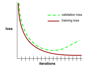
See Generalization in Machine Learning Crash Course for more information.
generalized linear model
A generalization of least squares regression models, which are based on Gaussian noise, to other types of models based on other types of noise, such as Poisson noise or categorical noise. Examples of generalized linear models include:
- logistic regression
- multi-class regression
- least squares regression
The parameters of a generalized linear model can be found through convex optimization.
Generalized linear models exhibit the following properties:
- The average prediction of the optimal least squares regression model is equal to the average label on the training data.
- The average probability predicted by the optimal logistic regression model is equal to the average label on the training data.
The power of a generalized linear model is limited by its features. Unlike a deep model, a generalized linear model cannot "learn new features."
generated text
#generativeAI
In general, the text that an ML model outputs. When evaluating large language models, some metrics compare generated text against reference text. For example, suppose you are trying to determine how effectively an ML model translates from French to Dutch. In this case:
- The generated text is the Dutch translation that the ML model outputs.
- The reference text is the Dutch translation that a human translator (or software) creates.
Note that some evaluation strategies don't involve reference text.
generative adversarial network (GAN)
A system to create new data in which a generator creates data and a discriminator determines whether that created data is valid or invalid.
See the Generative Adversarial Networks course for more information.
generative agents (simulacra)
#agent
Agents endowed with unique personas, memories, and routines that simulate realistic human behavior.
See Generative Agents: Interactive Simulacra of Human Behavior for details.
generative AI
#generativeAI
An emerging transformative field with no formal definition. That said, most experts agree that generative AI models can create ("generate") content that is all of the following:
- complex
- coherent
- original
Examples of generative AI include:
- Large language models, which can generate sophisticated original text and answer questions.
- Image generation model, which can produce unique images.
- Audio and music generation models, which can compose original music or generate realistic speech.
- Video generation models, which can generate original videos.
Some earlier technologies, including LSTMs and RNNs, can also generate original and coherent content. Some experts view these earlier technologies as generative AI, while others feel that true generative AI requires more complex output than those earlier technologies can produce.
Contrast with predictive ML.
generative model
Practically speaking, a model that does either of the following:
- Creates (generates) new examples from the training dataset. For example, a generative model could create poetry after training on a dataset of poems. The generator part of a generative adversarial network falls into this category.
- Determines the probability that a new example comes from the training set, or was created from the same mechanism that created the training set. For example, after training on a dataset consisting of English sentences, a generative model could determine the probability that new input is a valid English sentence.
A generative model can theoretically discern the distribution of examples or particular features in a dataset. That is:
p(examples)
Unsupervised learning models are generative.
Contrast with discriminative models.
generator
The subsystem within a generative adversarial network that creates new examples.
Contrast with discriminative model.
gini impurity
#df
#Metric
A metric similar to entropy. Splitters use values derived from either gini impurity or entropy to compose conditions for classification decision trees. Information gain is derived from entropy. No universally accepted equivalent term for the metric derived from gini impurity exists; however, this unnamed metric is just as important as information gain.
Gini impurity is also called gini index, or simply gini.
Click the icon for mathematical details about gini impurity.
Gini impurity is the probability of misclassifying a new piece of data taken from the same distribution. The gini impurity of a set with two possible values "0" and "1" (for example, the labels in a binary classification problem) is calculated from the following formula:
I = 1 - (p2 + q2) = 1 - (p2 + (1-p)2)
where:
- I is the gini impurity.
- p is the fraction of "1" examples.
- q is the fraction of "0" examples. Note that q = 1-p
For example, consider the following dataset:
- 100 labels (0.25 of the dataset) contain the value "1"
- 300 labels (0.75 of the dataset) contain the value "0"
Therefore, the gini impurity is:
- p = 0.25
- q = 0.75
- I = 1 - (0.252 + 0.752) = 0.375
Consequently, a random label from the same dataset would have a 37.5% chance of being misclassified, and a 62.5% chance of being properly classified.
A perfectly balanced label (for example, 200 "0"s and 200 "1"s) would have a gini impurity of 0.5. A highly imbalanced label would have a gini impurity close to 0.0.
golden dataset
A set of manually curated data that captures ground truth. Teams can use one or more golden datasets to evaluate a model's quality.
Some golden datasets capture different subdomains of ground truth. For example, a golden dataset for image classification might capture lighting conditions and image resolution.
golden response
#generativeAI
A response known to be good. For example, given the following prompt:
2 + 2
The golden response is hopefully:
4
Click here for notes about golden response and reference text.
Some evaluation metrics, such as ROUGE, compare reference text to a model's generated text. When there is a single right answer to a prompt, the golden response typically serves as the reference text.
Some prompts have no one right answer. For example, the prompt Summarize this document would likely have many right answers. For such prompts, reference text is often impractical because a model can generate a very wide range of possible summaries. However, a golden response might be helpful in this situation. For example, a golden response containing a good document summary can help train an autorater to discover patterns of good document summaries.
Google AI Studio
A Google tool providing a user-friendly interface for experimenting with and building applications using Google's large language models. See the Google AI Studio home page for details.
GPT (Generative Pre-trained Transformer)
#generativeAI
A family of Transformer-based large language models developed by OpenAI.
GPT variants can apply to multiple modalities, including:
- image generation (for example, ImageGPT)
- text-to-image generation (for example, DALL-E).
gradient
The vector of partial derivatives with respect to all of the independent variables. In machine learning, the gradient is the vector of partial derivatives of the model function. The gradient points in the direction of steepest ascent.
gradient accumulation
A backpropagation technique that updates the parameters only once per epoch rather than once per iteration. After processing each mini-batch, gradient accumulation simply updates a running total of gradients. Then, after processing the last mini-batch in the epoch, the system finally updates the parameters based on the total of all gradient changes.
Gradient accumulation is useful when the batch size is very large compared to the amount of available memory for training. When memory is an issue, the natural tendency is to reduce batch size. However, reducing the batch size in normal backpropagation increases the number of parameter updates. Gradient accumulation enables the model to avoid memory issues but still train efficiently.
gradient boosted (decision) trees (GBT)
#df
A type of decision forest in which:
- Training relies on gradient boosting.
- The weak model is a decision tree.
See Gradient Boosted Decision Trees in the Decision Forests course for more information.
gradient boosting
#df
A training algorithm where weak models are trained to iteratively improve the quality (reduce the loss) of a strong model. For example, a weak model could be a linear or small decision tree model. The strong model becomes the sum of all the previously trained weak models.
In the simplest form of gradient boosting, at each iteration, a weak model is trained to predict the loss gradient of the strong model. Then, the strong model's output is updated by subtracting the predicted gradient, similar to gradient descent.
$$F_{0} = 0$$ $$F_{i+1} = F_i - \xi f_i $$
where:
- $F_{0}$ is the starting strong model.
- $F_{i+1}$ is the next strong model.
- $F_{i}$ is the current strong model.
- $\xi$ is a value between 0.0 and 1.0 called shrinkage, which is analogous to the learning rate in gradient descent.
- $f_{i}$ is the weak model trained to predict the loss gradient of $F_{i}$.
Modern variations of gradient boosting also include the second derivative (Hessian) of the loss in their computation.
Decision trees are commonly used as weak models in gradient boosting. See gradient boosted (decision) trees.
gradient clipping
A commonly used mechanism to mitigate the exploding gradient problem by artificially limiting (clipping) the maximum value of gradients when using gradient descent to train a model.
gradient descent
#fundamentals
A mathematical technique to minimize loss. Gradient descent iteratively adjusts weights and biases, gradually finding the best combination to minimize loss.
Gradient descent is older—much, much older—than machine learning.
See the Linear regression: Gradient descent in Machine Learning Crash Course for more information.
graph
#TensorFlow
In TensorFlow, a computation specification. Nodes in the graph represent operations. Edges are directed and represent passing the result of an operation (a Tensor) as an operand to another operation. Use TensorBoard to visualize a graph.
graph execution
#TensorFlow
A TensorFlow programming environment in which the program first constructs a graph and then executes all or part of that graph. Graph execution is the default execution mode in TensorFlow 1.x.
Contrast with eager execution.
greedy policy
In reinforcement learning, a policy that always chooses the action with the highest expected return.
groundedness
A property of a model whose output is based on (is "grounded on") specific source material. For example, suppose you provide an entire physics textbook as input ("context") to a large language model. Then, you prompt that large language model with a physics question. If the model's response reflects information in that textbook, then that model is grounded on that textbook.
Note that a grounded model is not always a factual model. For example, the input physics textbook could contain mistakes.
grounding
The process of basing all or part of an LLM's response on information retrieved from one or more trusted sources. For example, suppose a user prompts an LLM for today's weather forecast in Berlin. The LLM might ground the response on information it gathers from the European Centre for Medium-Range Weather Forecasts.
Retrieval-augmented generation (RAG) is a common grounding technique.
ground truth
#fundamentals
Reality.
The thing that actually happened.
For example, consider a binary classification model that predicts whether a student in their first year of university will graduate within six years. Ground truth for this model is whether or not that student actually graduated within six years.
Click the icon for additional notes.
We assess model quality against ground truth. However, ground truth is not always completely, well, truthful. For example, consider the following examples of potential imperfections in ground truth:
- In the graduation example, are we certain that the graduation records for each student are always correct? Is the university's record-keeping flawless?
- Suppose the label is a floating-point value measured by instruments (for example, barometers). How can we be sure that each instrument is calibrated identically or that each reading was taken under the same circumstances?
- If the label is a matter of human opinion, how can we be sure that each human rater is evaluating events in the same way? To improve consistency, expert human raters sometimes intervene.
group attribution bias
#responsible
Assuming that what is true for an individual is also true for everyone in that group. The effects of group attribution bias can be exacerbated if a convenience sampling is used for data collection. In a non-representative sample, attributions may be made that don't reflect reality.
See also out-group homogeneity bias and in-group bias. Also, see Fairness: Types of bias in Machine Learning Crash Course for more information.
guardrails
Any software or process that prevents harm to humans or systems. Harm can take many forms, including preventing data leaks or unauthorized access, or ensuring that an LLM's responses don't contain offensive material.
H
hallucination
#generativeAI
The production of plausible-seeming but factually incorrect output by a generative AI model that purports to be making an assertion about the real world. For example, a generative AI model that claims that Barack Obama died in 1865 is hallucinating.
hashing
In machine learning, a mechanism for bucketing categorical data, particularly when the number of categories is large, but the number of categories actually appearing in the dataset is comparatively small.
For example, Earth is home to about 73,000 tree species. You could represent each of the 73,000 tree species in 73,000 separate categorical buckets. Alternatively, if only 200 of those tree species actually appear in a dataset, you could use hashing to divide tree species into perhaps 500 buckets.
A single bucket could contain multiple tree species. For example, hashing could place baobab and red maple—two genetically dissimilar species—into the same bucket. Regardless, hashing is still a good way to map large categorical sets into the selected number of buckets. Hashing turns a categorical feature having a large number of possible values into a much smaller number of values by grouping values in a deterministic way.
See Categorical data: Vocabulary and one-hot encoding in Machine Learning Crash Course for more information.
heuristic
A simple and quickly implemented solution to a problem. For example, "With a heuristic, we achieved 86% accuracy. When we switched to a deep neural network, accuracy went up to 98%."
#fundamentals
A layer in a neural network between the input layer (the features) and the output layer (the prediction). Each hidden layer consists of one or more neurons. For example, the following neural network contains two hidden layers, the first with three neurons and the second with two neurons:
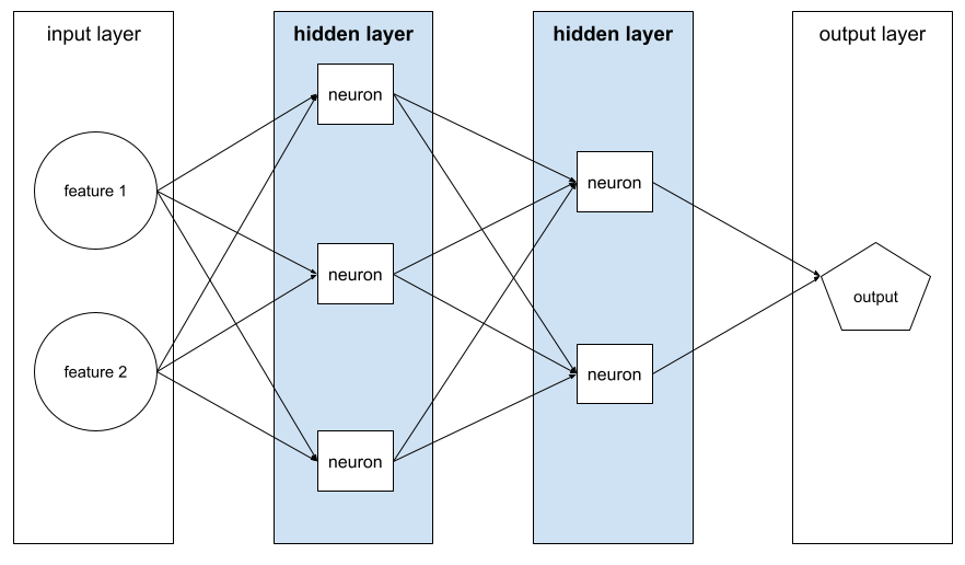
A deep neural network contains more than one hidden layer. For example, the preceding illustration is a deep neural network because the model contains two hidden layers.
See Neural networks: Nodes and hidden layers in Machine Learning Crash Course for more information.
hierarchical clustering
#clustering
A category of clustering algorithms that create a tree of clusters. Hierarchical clustering is well-suited to hierarchical data, such as botanical taxonomies. There are two types of hierarchical clustering algorithms:
- Agglomerative clustering first assigns every example to its own cluster, and iteratively merges the closest clusters to create a hierarchical tree.
- Divisive clustering first groups all examples into one cluster and then iteratively divides the cluster into a hierarchical tree.
Contrast with centroid-based clustering.
See Clustering algorithms in the Clustering course for more information.
hill climbing
An algorithm for iteratively improving ("walking uphill") an ML model until the model stops improving ("reaches the top of a hill"). The general form of the algorithm is as follows:
- Build a starting model.
- Create new candidate models by making small adjustments to the way you train or fine-tune. This might entail working with a slightly different training set or different hyperparameters.
- Evaluate the new candidate models and take one of the
following actions:
- If a candidate model outperforms the starting model, then that candidate model becomes the new starting model. In this case, repeat Steps 1, 2, and 3.
- If no model outperforms the starting model, then you've reached the top of the hill and should stop iterating.
See Deep Learning Tuning Playbook for guidance on hyperparameter tuning. See the Data modules of Machine Learning Crash Course for guidance on feature engineering.
hinge loss
#Metric
A family of loss functions for classification designed to find the decision boundary as distant as possible from each training example, thus maximizing the margin between examples and the boundary. KSVMs use hinge loss (or a related function, such as squared hinge loss). For binary classification, the hinge loss function is defined as follows:
$$\text{loss} = \text{max}(0, 1 - (y * y'))$$
where y is the true label, either -1 or +1, and y' is the raw output of the classification model:
$$y' = b + w_1x_1 + w_2x_2 + … w_nx_n$$
Consequently, a plot of hinge loss versus (y * y') looks as follows:
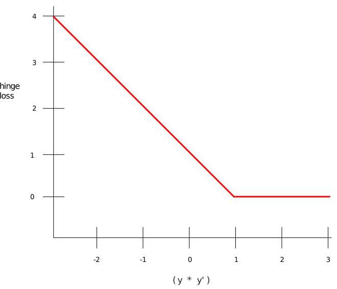
historical bias
#responsible
A type of bias that already exists in the world and has made its way into a dataset. These biases have a tendency to reflect existing cultural stereotypes, demographic inequalities, and prejudices against certain social groups.
For example, consider a classification model that predicts whether or not a loan applicant will default on their loan, which was trained on historical loan-default data from the 1980s from local banks in two different communities. If past applicants from Community A were six times more likely to default on their loans than applicants from Community B, the model might learn a historical bias resulting in the model being less likely to approve loans in Community A, even if the historical conditions that resulted in that community's higher default rates were no longer relevant.
See Fairness: Types of bias in Machine Learning Crash Course for more information.
holdout data
Examples intentionally not used ("held out") during training. The validation dataset and test dataset are examples of holdout data. Holdout data helps evaluate your model's ability to generalize to data other than the data it was trained on. The loss on the holdout set provides a better estimate of the loss on an unseen dataset than does the loss on the training set.
host
#TensorFlow
#GoogleCloud
When training an ML model on accelerator chips (GPUs or TPUs), the part of the system that controls both of the following:
- The overall flow of the code.
- The extraction and transformation of the input pipeline.
The host typically runs on a CPU, not on an accelerator chip; the device manipulates tensors on the accelerator chips.
human evaluation
#generativeAI
A process in which people judge the quality of an ML model's output; for example, having bilingual people judge the quality of an ML translation model. Human evaluation is particularly useful for judging models that have no one right answer.
Contrast with automatic evaluation and autorater evaluation.
human in the loop (HITL)
#generativeAI
A loosely-defined idiom that could mean either of the following:
- A policy of viewing generative AI output critically or skeptically.
- A strategy or system for ensuring that people help shape, evaluate, and refine a model's behavior. Keeping a human in the loop enables an AI to benefit from both machine intelligence and human intelligence. For example, a system in which an AI generates code which software engineers then review is a human-in-the-loop system.
hyperparameter
#fundamentals
The variables that you or a hyperparameter tuning service adjust during successive runs of training a model. For example, learning rate is a hyperparameter. You could set the learning rate to 0.01 before one training session. If you determine that 0.01 is too high, you could perhaps set the learning rate to 0.003 for the next training session.
In contrast, parameters are the various weights and bias that the model learns during training.
See Linear regression: Hyperparameters in Machine Learning Crash Course for more information.
hyperplane
A boundary that separates a space into two subspaces. For example, a line is a hyperplane in two dimensions and a plane is a hyperplane in three dimensions. More typically in machine learning, a hyperplane is the boundary separating a high-dimensional space. Kernel Support Vector Machines use hyperplanes to separate positive classes from negative classes, often in a very high-dimensional space.
I
i.i.d.
Abbreviation for independently and identically distributed.
image recognition
A process that classifies object(s), pattern(s), or concept(s) in an image. Image recognition is also known as image classification.
imbalanced dataset
Synonym for class-imbalanced dataset.
implicit bias
#responsible
Automatically making an association or assumption based on one's mind models and memories. Implicit bias can affect the following:
- How data is collected and classified.
- How machine learning systems are designed and developed.
For example, when building a classification model to identify wedding photos, an engineer may use the presence of a white dress in a photo as a feature. However, white dresses have been customary only during certain eras and in certain cultures.
See also confirmation bias.
imputation
Short form of value imputation.
incompatibility of fairness metrics
#responsible
#Metric
The idea that some notions of fairness are mutually incompatible and cannot be satisfied simultaneously. As a result, there is no single universal metric for quantifying fairness that can be applied to all ML problems.
While this may seem discouraging, incompatibility of fairness metrics doesn't imply that fairness efforts are fruitless. Instead, it suggests that fairness must be defined contextually for a given ML problem, with the goal of preventing harms specific to its use cases.
See "On the (im)possibility of fairness" for a more detailed discussion of the incompatibility of fairness metrics.
in-context learning
#generativeAI
Synonym for few-shot prompting.
independently and identically distributed (i.i.d)
#fundamentals
Data drawn from a distribution that doesn't change, and where each value drawn doesn't depend on values that have been drawn previously. An i.i.d. is the ideal gas of machine learning—a useful mathematical construct but almost never exactly found in the real world. For example, the distribution of visitors to a web page may be i.i.d. over a brief window of time; that is, the distribution doesn't change during that brief window and one person's visit is generally independent of another's visit. However, if you expand that window of time, seasonal differences in the web page's visitors may appear.
See also nonstationarity.
individual fairness
#responsible
#Metric
A fairness metric that checks whether similar individuals are classified similarly. For example, Brobdingnagian Academy might want to satisfy individual fairness by ensuring that two students with identical grades and standardized test scores are equally likely to gain admission.
Note that individual fairness relies entirely on how you define "similarity" (in this case, grades and test scores), and you can run the risk of introducing new fairness problems if your similarity metric misses important information (such as the rigor of a student's curriculum).
See "Fairness Through Awareness" for a more detailed discussion of individual fairness.
inference
#fundamentals
#generativeAI
In traditional machine learning, the process of making predictions by applying a trained model to unlabeled examples. See Supervised Learning in the Intro to ML course to learn more.
In large language models, inference is the process of using a trained model to generate a response to an input prompt.
Inference has a somewhat different meaning in statistics. See the Wikipedia article on statistical inference for details.
inference path
#df
In a decision tree, during inference, the route a particular example takes from the root to other conditions, terminating with a leaf. For example, in the following decision tree, the thicker arrows show the inference path for an example with the following feature values:
- x = 7
- y = 12
- z = -3
The inference path in the following illustration travels through three
conditions before reaching the leaf (Zeta).
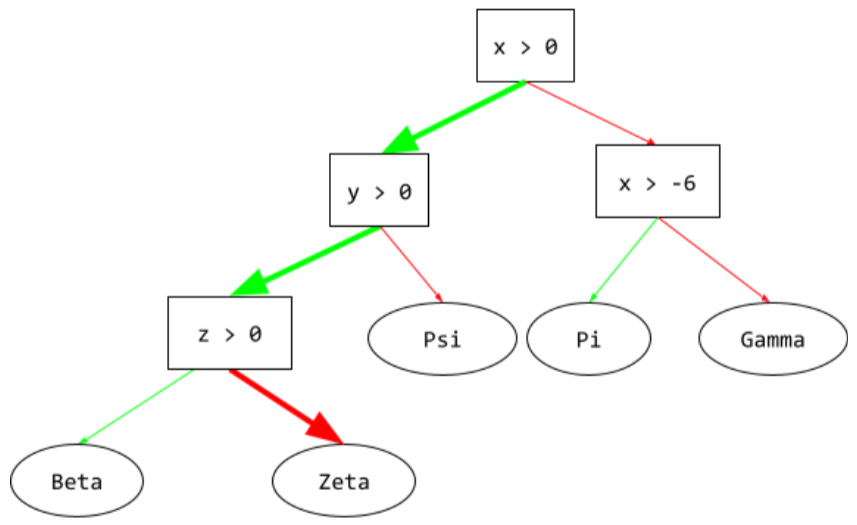
The three thick arrows show the inference path.
See Decision trees in the Decision Forests course for more information.
information gain
#df
#Metric
In decision forests, the difference between a node's entropy and the weighted (by number of examples) sum of the entropy of its children nodes. A node's entropy is the entropy of the examples in that node.
For example, consider the following entropy values:
- entropy of parent node = 0.6
- entropy of one child node with 16 relevant examples = 0.2
- entropy of another child node with 24 relevant examples = 0.1
So 40% of the examples are in one child node and 60% are in the other child node. Therefore:
- weighted entropy sum of child nodes = (0.4 * 0.2) + (0.6 * 0.1) = 0.14
So, the information gain is:
- information gain = entropy of parent node - weighted entropy sum of child nodes
- information gain = 0.6 - 0.14 = 0.46
Most splitters seek to create conditions that maximize information gain.
in-group bias
#responsible
Showing partiality to one's own group or own characteristics. If testers or raters consist of the machine learning developer's friends, family, or colleagues, then in-group bias may invalidate product testing or the dataset.
In-group bias is a form of group attribution bias. See also out-group homogeneity bias.
See Fairness: Types of bias in Machine Learning Crash Course for more information.
input generator
A mechanism by which data is loaded into a neural network.
An input generator can be thought of as a component responsible for processing raw data into tensors which are iterated over to generate batches for training, evaluation, and inference.
input layer
#fundamentals
The layer of a neural network that holds the feature vector. That is, the input layer provides examples for training or inference. For example, the input layer in the following neural network consists of two features:
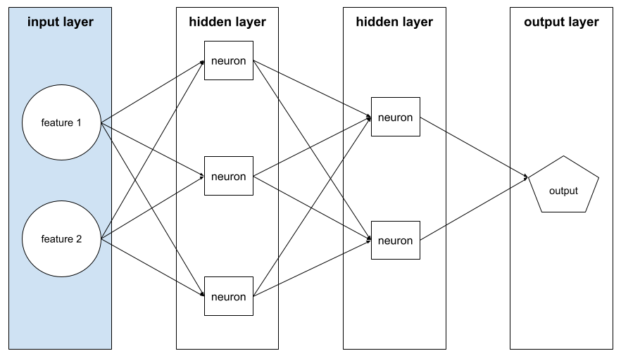
in-set condition
#df
In a decision tree, a condition that tests for the presence of one item in a set of items. For example, the following is an in-set condition:
house-style in [tudor, colonial, cape]
During inference, if the value of the house-style feature
is tudor or colonial or cape, then this condition evaluates to Yes. If
the value of the house-style feature is something else (for example, ranch),
then this condition evaluates to No.
In-set conditions usually lead to more efficient decision trees than conditions that test one-hot encoded features.
instance
Synonym for example.
instruction tuning
#generativeAI
A form of fine-tuning that improves a generative AI model's ability to follow instructions. Instruction tuning involves training a model on a series of instruction prompts, typically covering a wide variety of tasks. The resulting instruction-tuned model then tends to generate useful responses to zero-shot prompts across a variety of tasks.
Compare and contrast with:
interpretability
#fundamentals
The ability to explain or to present an ML model's reasoning in understandable terms to a human.
Most linear regression models, for example, are highly interpretable. (You merely need to look at the trained weights for each feature.) Decision forests are also highly interpretable. Some models, however, require sophisticated visualization to become interpretable.
You can use the Learning Interpretability Tool (LIT) to interpret ML models.
inter-rater agreement
#Metric
A measurement of how often human raters agree when doing a task. If raters disagree, the task instructions may need to be improved. Also sometimes called inter-annotator agreement or inter-rater reliability. See also Cohen's kappa, which is one of the most popular inter-rater agreement measurements.
See Categorical data: Common issues in Machine Learning Crash Course for more information.
intersection over union (IoU)
The intersection of two sets divided by their union. In machine-learning image-detection tasks, IoU is used to measure the accuracy of the model's predicted bounding box with respect to the ground-truth bounding box. In this case, the IoU for the two boxes is the ratio between the overlapping area and the total area, and its value ranges from 0 (no overlap of predicted bounding box and ground-truth bounding box) to 1 (predicted bounding box and ground-truth bounding box have the exact same coordinates).
For example, in the image below:
- The predicted bounding box (the coordinates delimiting where the model predicts the night table in the painting is located) is outlined in purple.
- The ground-truth bounding box (the coordinates delimiting where the night table in the painting is actually located) is outlined in green.
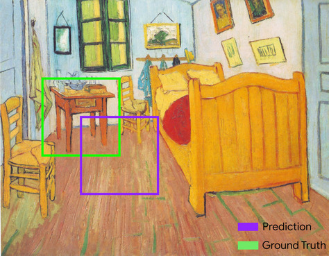
Here, the intersection of the bounding boxes for prediction and ground truth (below left) is 1, and the union of the bounding boxes for prediction and ground truth (below right) is 7, so the IoU is \(\frac{1}{7}\).
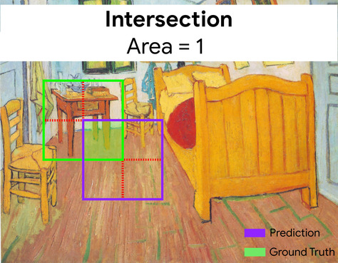
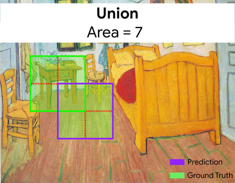
IoU
Abbreviation for intersection over union.
item matrix
In recommendation systems, a matrix of embedding vectors generated by matrix factorization that holds latent signals about each item. Each row of the item matrix holds the value of a single latent feature for all items. For example, consider a movie recommendation system. Each column in the item matrix represents a single movie. The latent signals might represent genres, or might be harder-to-interpret signals that involve complex interactions among genre, stars, movie age, or other factors.
The item matrix has the same number of columns as the target matrix that is being factorized. For example, given a movie recommendation system that evaluates 10,000 movie titles, the item matrix will have 10,000 columns.
items
In a recommendation system, the entities that a system recommends. For example, videos are the items that a video store recommends, while books are the items that a bookstore recommends.
iteration
#fundamentals
A single update of a model's parameters—the model's weights and biases—during training. The batch size determines how many examples the model processes in a single iteration. For instance, if the batch size is 20, then the model processes 20 examples before adjusting the parameters.
When training a neural network, a single iteration involves the following two passes:
- A forward pass to evaluate loss on a single batch.
- A backward pass (backpropagation) to adjust the model's parameters based on the loss and the learning rate.
See Gradient descent in Machine Learning Crash Course for more information.
J
JAX
An array computing library, bringing together XLA (Accelerated Linear Algebra) and automatic differentiation for high-performance numerical computing. JAX provides a simple and powerful API for writing accelerated numerical code with composable transformations. JAX provides features such as:
grad(automatic differentiation)jit(just-in-time compilation)vmap(automatic vectorization or batching)pmap(parallelization)
JAX is a language for expressing and composing transformations of numerical code, analogous—but much larger in scope—to Python's NumPy library. (In fact, the .numpy library under JAX is a functionally equivalent, but entirely rewritten version of the Python NumPy library.)
JAX is particularly well-suited for speeding up many machine learning tasks by transforming the models and data into a form suitable for parallelism across GPU and TPU accelerator chips.
Flax, Optax, Pax, and many other libraries are built on the JAX infrastructure.
K
Keras
A popular Python machine learning API. Keras runs on several deep learning frameworks, including TensorFlow, where it is made available as tf.keras.
Kernel Support Vector Machines (KSVMs)
A classification algorithm that seeks to maximize the margin between positive and negative classes by mapping input data vectors to a higher dimensional space. For example, consider a classification problem in which the input dataset has a hundred features. To maximize the margin between positive and negative classes, a KSVM could internally map those features into a million-dimension space. KSVMs uses a loss function called hinge loss.
keypoints
The coordinates of particular features in an image. For example, for an image recognition model that distinguishes flower species, keypoints might be the center of each petal, the stem, the stamen, and so on.
k-fold cross validation
An algorithm for predicting a model's ability to generalize to new data. The k in k-fold refers to the number of equal groups you divide a dataset's examples into; that is, you train and test your model k times. For each round of training and testing, a different group is the test set, and all remaining groups become the training set. After k rounds of training and testing, you calculate the mean and standard deviation of the chosen test metric(s).
For example, suppose your dataset consists of 120 examples. Further suppose, you decide to set k to 4. Therefore, after shuffling the examples, you divide the dataset into four equal groups of 30 examples and conduct four training and testing rounds:
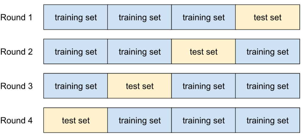
For example, Mean Squared Error (MSE) might be the most meaningful metric for a linear regression model. Therefore, you would find the mean and standard deviation of the MSE across all four rounds.
k-means
#clustering
A popular clustering algorithm that groups examples in unsupervised learning. The k-means algorithm basically does the following:
- Iteratively determines the best k center points (known as centroids).
- Assigns each example to the closest centroid. Those examples nearest the same centroid belong to the same group.
The k-means algorithm picks centroid locations to minimize the cumulative square of the distances from each example to its closest centroid.
For example, consider the following plot of dog height to dog width:
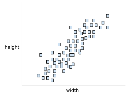
If k=3, the k-means algorithm will determine three centroids. Each example is assigned to its closest centroid, yielding three groups:
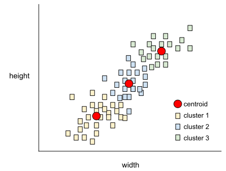
Imagine that a manufacturer wants to determine the ideal sizes for small, medium, and large sweaters for dogs. The three centroids identify the mean height and mean width of each dog in that cluster. So, the manufacturer should probably base sweater sizes on those three centroids. Note that the centroid of a cluster is typically not an example in the cluster.
The preceding illustrations shows k-means for examples with only two features (height and width). Note that k-means can group examples across many features.
See What is k-means clustering? in the Clustering course for more information.
#clustering
A clustering algorithm closely related to k-means. The practical difference between the two is as follows:
- In k-means, centroids are determined by minimizing the sum of the squares of the distance between a centroid candidate and each of its examples.
- In k-median, centroids are determined by minimizing the sum of the distance between a centroid candidate and each of its examples.
Note that the definitions of distance are also different:
- k-means relies on the Euclidean distance from the centroid to an example. (In two dimensions, the Euclidean distance means using the Pythagorean theorem to calculate the hypotenuse.) For example, the k-means distance between (2,2) and (5,-2) would be:
$$ {\text{Euclidean distance}} = {\sqrt {(2-5)^2 + (2--2)^2}} = 5 $$
- k-median relies on the Manhattan distance from the centroid to an example. This distance is the sum of the absolute deltas in each dimension. For example, the k-median distance between (2,2) and (5,-2) would be:
$$ {\text{Manhattan distance}} = \lvert 2-5 \rvert + \lvert 2--2 \rvert = 7 $$
L
L0 regularization
#fundamentals
A type of regularization that penalizes the total number of nonzero weights in a model. For example, a model having 11 nonzero weights would be penalized more than a similar model having 10 nonzero weights.
L0 regularization is sometimes called L0-norm regularization.
Click the icon for additional notes.
L0 regularization is generally impractical in large models because L0 regularization turns training into a convex optimization problem.
L1 loss
#fundamentals
#Metric
A loss function that calculates the absolute value of the difference between actual label values and the values that a model predicts. For example, here's the calculation of L1 loss for a batch of five examples:
| Actual value of example | Model's predicted value | Absolute value of delta |
|---|---|---|
| 7 | 6 | 1 |
| 5 | 4 | 1 |
| 8 | 11 | 3 |
| 4 | 6 | 2 |
| 9 | 8 | 1 |
| 8 = L1 loss | ||
L1 loss is less sensitive to outliers than L2 loss.
The Mean Absolute Error is the average L1 loss per example.
Click the icon to see the formal math.
$$ L_1 loss = \sum_{i=0}^n | y_i - \hat{y}_i |$$
where:
- $n$ is the number of examples.
- $y$ is the actual value of the label.
- $\hat{y}$ is the value that the model predicts for $y$.
See Linear regression: Loss in Machine Learning Crash Course for more information.
L1 regularization
#fundamentals
A type of regularization that penalizes weights in proportion to the sum of the absolute value of the weights. L1 regularization helps drive the weights of irrelevant or barely relevant features to exactly 0. A feature with a weight of 0 is effectively removed from the model.
Contrast with L2 regularization.
L2 loss
#fundamentals
#Metric
A loss function that calculates the square of the difference between actual label values and the values that a model predicts. For example, here's the calculation of L2 loss for a batch of five examples:
| Actual value of example | Model's predicted value | Square of delta |
|---|---|---|
| 7 | 6 | 1 |
| 5 | 4 | 1 |
| 8 | 11 | 9 |
| 4 | 6 | 4 |
| 9 | 8 | 1 |
| 16 = L2 loss | ||
Due to squaring, L2 loss amplifies the influence of outliers. That is, L2 loss reacts more strongly to bad predictions than L1 loss. For example, the L1 loss for the preceding batch would be 8 rather than 16. Notice that a single outlier accounts for 9 of the 16.
Regression models typically use L2 loss as the loss function.
The Mean Squared Error is the average L2 loss per example. Squared loss is another name for L2 loss.
Click the icon to see the formal math.
$$ L_2 loss = \sum_{i=0}^n {(y_i - \hat{y}_i)}^2$$
where:
- $n$ is the number of examples.
- $y$ is the actual value of the label.
- $\hat{y}$ is the value that the model predicts for $y$.
See Logistic regression: Loss and regularization in Machine Learning Crash Course for more information.
L2 regularization
#fundamentals
A type of regularization that penalizes weights in proportion to the sum of the squares of the weights. L2 regularization helps drive outlier weights (those with high positive or low negative values) closer to 0 but not quite to 0. Features with values very close to 0 remain in the model but don't influence the model's prediction very much.
L2 regularization always improves generalization in linear models.
Contrast with L1 regularization.
See Overfitting: L2 regularization in Machine Learning Crash Course for more information.
label
#fundamentals
In supervised machine learning, the "answer" or "result" portion of an example.
Each labeled example consists of one or more features and a label. For example, in a spam detection dataset, the label would probably be either "spam" or "not spam." In a rainfall dataset, the label might be the amount of rain that fell during a certain period.
See Supervised Learning in Introduction to Machine Learning for more information.
labeled example
#fundamentals
An example that contains one or more features and a label. For example, the following table shows three labeled examples from a house valuation model, each with three features and one label:
| Number of bedrooms | Number of bathrooms | House age | House price (label) |
|---|---|---|---|
| 3 | 2 | 15 | $345,000 |
| 2 | 1 | 72 | $179,000 |
| 4 | 2 | 34 | $392,000 |
In supervised machine learning, models train on labeled examples and make predictions on unlabeled examples.
Contrast labeled example with unlabeled examples.
See Supervised Learning in Introduction to Machine Learning for more information.
label leakage
A model design flaw in which a feature is a proxy for the
label. For example, consider a
binary classification model that predicts
whether or not a prospective customer will purchase a particular product.
Suppose that one of the features for the model is a Boolean named
SpokeToCustomerAgent. Further suppose that a customer agent is only
assigned after the prospective customer has actually purchased the
product. During training, the model will quickly learn the association
between SpokeToCustomerAgent and the label.
See Monitoring pipelines in Machine Learning Crash Course for more information.
lambda
#fundamentals
Synonym for regularization rate.
Lambda is an overloaded term. Here we're focusing on the term's definition within regularization.
LaMDA (Language Model for Dialogue Applications)
A Transformer-based large language model developed by Google trained on a large dialogue dataset that can generate realistic conversational responses.
LaMDA: our breakthrough conversation technology provides an overview.
landmarks
Synonym for keypoints.
language model
A model that estimates the probability of a token or sequence of tokens occurring in a longer sequence of tokens.
Click the icon for additional notes.
Though counterintuitive, many models that evaluate text are not language models. For example, text classification models and sentiment analysis models are not language models.
See What is a language model? in Machine Learning Crash Course for more information.
large language model
#generativeAI
At a minimum, a language model having a very high number of parameters. More informally, any Transformer-based language model, such as Gemini or GPT.
See Large language models (LLMs) in Machine Learning Crash Course for more information.
latency
#generativeAI
The time it takes for a model to process input and generate a response. A high latency response takes takes longer to generate than a low latency response.
Factors that influence latency of large language models include:
- Input and output token lengths
- Model complexity
- The infrastructure the model runs on
Optimizing for latency is crucial for creating responsive and user-friendly applications.
latent space
Synonym for embedding space.
layer
#fundamentals
A set of neurons in a neural network. Three common types of layers are as follows:
- The input layer, which provides values for all the features.
- One or more hidden layers, which find nonlinear relationships between the features and the label.
- The output layer, which provides the prediction.
For example, the following illustration shows a neural network with one input layer, two hidden layers, and one output layer:
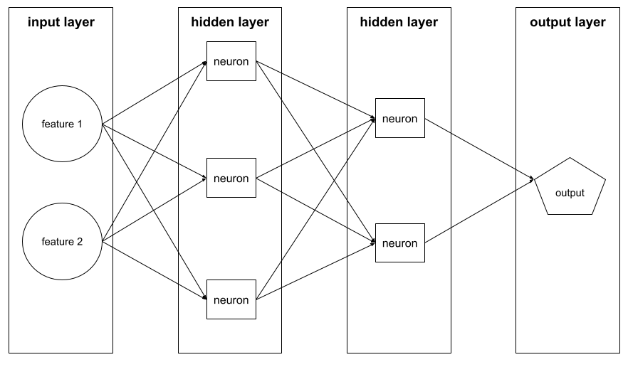
In TensorFlow, layers are also Python functions that take Tensors and configuration options as input and produce other tensors as output.
Layers API (tf.layers)
#TensorFlow
A TensorFlow API for constructing a deep neural network as a composition of layers. The Layers API lets you build different types of layers, such as:
tf.layers.Densefor a fully-connected layer.tf.layers.Conv2Dfor a convolutional layer.
The Layers API follows the Keras layers API conventions. That is, aside from a different prefix, all functions in the Layers API have the same names and signatures as their counterparts in the Keras layers API.
leaf
#df
Any endpoint in a decision tree. Unlike a condition, a leaf doesn't perform a test. Rather, a leaf is a possible prediction. A leaf is also the terminal node of an inference path.
For example, the following decision tree contains three leaves:
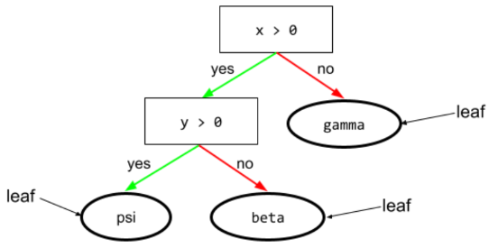
See Decision trees in the Decision Forests course for more information.
Learning Interpretability Tool (LIT)
A visual, interactive model-understanding and data visualization tool.
You can use open-source LIT to interpret models or to visualize text, image, and tabular data.
learning rate
#fundamentals
A floating-point number that tells the gradient descent algorithm how strongly to adjust weights and biases on each iteration. For example, a learning rate of 0.3 would adjust weights and biases three times more powerfully than a learning rate of 0.1.
Learning rate is a key hyperparameter. If you set the learning rate too low, training will take too long. If you set the learning rate too high, gradient descent often has trouble reaching convergence.
Click the icon for a more mathematical explanation.
During each iteration, the gradient descent algorithm multiplies the learning rate by the gradient. The resulting product is called the gradient step.
See Linear regression: Hyperparameters in Machine Learning Crash Course for more information.
least squares regression
A linear regression model trained by minimizing L2 Loss.
least-to-most prompting
A form of prompt chaining that divides complex problems into an ordered set of simpler problems. For example, here's a least-to-most prompting strategy for a certain problem:
- Divide a complex problem into an ordered list of simpler sub-problems. For this example, assume it is three sub-problems.
- Prompt 1: Ask the LLM to solve the first sub-problem. The LLM returns Response 1.
- Prompt 2: Integrate all or part of Response 1 into the prompt to solve the second sub-problem. The LLM returns Response 2.
- Prompt 3: Integrate all or part of Response 2 into the prompt to solve the third sub-problem. The LLM's response to Prompt 3 is the "final" answer to the initial complex problem.
Note that each step depends on the solution to the preceding step.
Contrast with tree-of-thought prompting.
Levenshtein Distance
#metric
An edit distance metric that calculates the fewest delete, insert, and substitute operations required to change one word to another. For example, the Levenshtein distance between the words "heart" and "darts" is three because the following three edits are the fewest changes to turn one word into the other:
- heart → deart (substitute "h" with "d")
- deart → dart (delete "e")
- dart → darts (insert "s")
Note that the preceding sequence isn't the only path of three edits.
linear
#fundamentals
A relationship between two or more variables that can be represented solely through addition and multiplication.
The plot of a linear relationship is a line.
Contrast with nonlinear.
linear model
#fundamentals
A model that assigns one weight per feature to make predictions. (Linear models also incorporate a bias.) In contrast, the relationship of features to predictions in deep models is generally nonlinear.
Linear models are usually easier to train and more interpretable than deep models. However, deep models can learn complex relationships between features.
Linear regression and logistic regression are two types of linear models.
Click the icon to see the math.
A linear model follows this formula:
$$y' = b + w_1x_1 + w_2x_2 + … w_nx_n$$
where:
- y' is the raw prediction. (In certain kinds of linear models, this raw prediction will be further modified. For example, see logistic regression.)
- b is the bias.
- w is a weight, so w1 is the weight of the first feature, w2 is the weight of the second feature, and so on.
- x is a feature, so x1 is the value of the first feature, x2 is the value of the second feature, and so on.
For example, suppose a linear model for three features learns the following bias and weights:
- b = 7
- w1 = -2.5
- w2 = -1.2
- w3 = 1.4
Therefore, given three features (x1, x2, and x3), the linear model uses the following equation to generate each prediction:
y' = 7 + (-2.5)(x1) + (-1.2)(x2) + (1.4)(x3)
Suppose a particular example contains the following values:
- x1 = 4
- x2 = -10
- x3 = 5
Plugging those values into the formula yields a prediction for this example:
y' = 7 + (-2.5)(4) + (-1.2)(-10) + (1.4)(5)
y' = 16
Linear models include not only models that use only a linear equation to make predictions but also a broader set of models that use a linear equation as just one component of the formula that makes predictions. For example, logistic regression post-processes the raw prediction (y') to produce a final prediction value between 0 and 1, exclusively.
linear regression
#fundamentals
A type of machine learning model in which both of the following are true:
- The model is a linear model.
- The prediction is a floating-point value. (This is the regression part of linear regression.)
Contrast linear regression with logistic regression. Also, contrast regression with classification.
See Linear regression in Machine Learning Crash Course for more information.
LIT
Abbreviation for the Learning Interpretability Tool (LIT), which was previously known as the Language Interpretability Tool.
LLM
#generativeAI
Abbreviation for large language model.
LLM evaluations (evals)
#generativeAI
#Metric
A set of metrics and benchmarks for assessing the performance of large language models (LLMs). At a high level, LLM evaluations:
- Help researchers identify areas where LLMs need improvement.
- Are useful in comparing different LLMs and identifying the best LLM for a particular task.
- Help ensure that LLMs are safe and ethical to use.
See Large language models (LLMs) in Machine Learning Crash Course for more information.
logistic regression
#fundamentals
A type of regression model that predicts a probability. Logistic regression models have the following characteristics:
- The label is categorical. The term logistic regression usually refers to binary logistic regression, that is, to a model that calculates probabilities for labels with two possible values. A less common variant, multinomial logistic regression, calculates probabilities for labels with more than two possible values.
- The loss function during training is Log Loss. (Multiple Log Loss units can be placed in parallel for labels with more than two possible values.)
- The model has a linear architecture, not a deep neural network. However, the remainder of this definition also applies to deep models that predict probabilities for categorical labels.
For example, consider a logistic regression model that calculates the probability of an input email being either spam or not spam. During inference, suppose the model predicts 0.72. Therefore, the model is estimating:
- A 72% chance of the email being spam.
- A 28% chance of the email not being spam.
A logistic regression model uses the following two-step architecture:
- The model generates a raw prediction (y') by applying a linear function of input features.
- The model uses that raw prediction as input to a sigmoid function, which converts the raw prediction to a value between 0 and 1, exclusive.
Like any regression model, a logistic regression model predicts a number. However, this number typically becomes part of a binary classification model as follows:
- If the predicted number is greater than the classification threshold, the binary classification model predicts the positive class.
- If the predicted number is less than the classification threshold, the binary classification model predicts the negative class.
See Logistic regression in Machine Learning Crash Course for more information.
logits
The vector of raw (non-normalized) predictions that a classification model generates, which is ordinarily then passed to a normalization function. If the model is solving a multi-class classification problem, logits typically become an input to the softmax function. The softmax function then generates a vector of (normalized) probabilities with one value for each possible class.
Log Loss
#fundamentals
The loss function used in binary logistic regression.
Click the icon to see the math.
The following formula calculates Log Loss:
$$\text{Log Loss} = \sum_{(x,y)\in D} -y\log(y') - (1 - y)\log(1 - y')$$
where:
- \((x,y)\in D\) is the dataset containing many labeled examples, which are \((x,y)\) pairs.
- \(y\) is the label in a labeled example. Since this is logistic regression, every value of \(y\) must either be 0 or 1.
- \(y'\) is the predicted value (somewhere between 0 and 1, exclusive), given the set of features in \(x\).
See Logistic regression: Loss and regularization in Machine Learning Crash Course for more information.
log-odds
#fundamentals
The logarithm of the odds of some event.
Click the icon to see the math.
If the event is a binary probability, then odds refers to the ratio of the probability of success (p) to the probability of failure (1-p). For example, suppose that a given event has a 90% probability of success and a 10% probability of failure. In this case, odds is calculated as follows:
$$ {\text{odds}} = \frac{\text{p}} {\text{(1-p)}} = \frac{.9} {.1} = {\text{9}} $$
The log-odds is simply the logarithm of the odds. By convention, "logarithm" refers to natural logarithm, but logarithm could actually be any base greater than 1. Sticking to convention, the log-odds of our example is therefore:
$$ {\text{log-odds}} = ln(9) ~= 2.2 $$
The log-odds function is the inverse of the sigmoid function.
Long Short-Term Memory (LSTM)
A type of cell in a recurrent neural network used to process sequences of data in applications such as handwriting recognition, machine translation, and image captioning. LSTMs address the vanishing gradient problem that occurs when training RNNs due to long data sequences by maintaining history in an internal memory state based on new input and context from previous cells in the RNN.
LoRA
#generativeAI
Abbreviation for Low-Rank Adaptability.
loss
#fundamentals
#Metric
During the training of a supervised model, a measure of how far a model's prediction is from its label.
A loss function calculates the loss.
See Linear regression: Loss in Machine Learning Crash Course for more information.
loss aggregator
A type of machine learning algorithm that improves the performance of a model by combining the predictions of multiple models and using those predictions to make a single prediction. As a result, a loss aggregator can reduce the variance of the predictions and improve the accuracy of the predictions.
loss curve
#fundamentals
A plot of loss as a function of the number of training iterations. The following plot shows a typical loss curve:
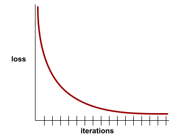
Loss curves can help you determine when your model is converging or overfitting.
Loss curves can plot all of the following types of loss:
See also generalization curve.
See Overfitting: Interpreting loss curves in Machine Learning Crash Course for more information.
loss function
#fundamentals
#Metric
During training or testing, a mathematical function that calculates the loss on a batch of examples. A loss function returns a lower loss for models that makes good predictions than for models that make bad predictions.
The goal of training is typically to minimize the loss that a loss function returns.
Many different kinds of loss functions exist. Pick the appropriate loss function for the kind of model you are building. For example:
- L2 loss (or Mean Squared Error) is the loss function for linear regression.
- Log Loss is the loss function for logistic regression.
loss surface
A graph of weight(s) versus loss. Gradient descent aims to find the weight(s) for which the loss surface is at a local minimum.
lost-in-the-middle effect
An LLM's tendency to use information from the start and end of a long context window more effectively than information from the middle. That is, given a long context, the lost-in-the-middle effect causes accuracy to be:
- Relatively high when the relevant information to form a response is near the beginning or end of the context.
- Relatively low when the relevant information to form a response is in the middle of the context.
The term comes from Lost in the Middle: How Language Models Use Long Contexts.
Low-Rank Adaptability (LoRA)
#generativeAI
A parameter-efficient technique for fine tuning that "freezes" the model's pre-trained weights (such that they can no longer be modified) and then inserts a small set of trainable weights into the model. This set of trainable weights (also known as "update matrixes") is considerably smaller than the base model and is therefore much faster to train.
LoRA provides the following benefits:
- Improves the quality of a model's predictions for the domain where the fine tuning is applied.
- Fine-tunes faster than techniques that require fine-tuning all of a model's parameters.
- Reduces the computational cost of inference by enabling concurrent serving of multiple specialized models sharing the same base model.
Click the icon to learn more about update matrixes in LoRA.
The update matrixes used in LoRA consist of rank decomposition matrixes, which are derived from the base model to help filter out noise and focus training on the most important features of the model.
LSTM
Abbreviation for Long Short-Term Memory.
M
#fundamentals
A program or system that trains a model from input data. The trained model can make useful predictions from new (never-before-seen) data drawn from the same distribution as the one used to train the model.
Machine learning also refers to the field of study concerned with these programs or systems.
See the Introduction to Machine Learning course for more information.
machine translation
#generativeAI
Using software (typically, a machine learning model) to convert text from one human language to another human language, for example, from English to Japanese.
majority class
#fundamentals
The more common label in a class-imbalanced dataset. For example, given a dataset containing 99% negative labels and 1% positive labels, the negative labels are the majority class.
Contrast with minority class.
See Datasets: Imbalanced datasets in Machine Learning Crash Course for more information.
manager agent
#agent
An agent that controls one or more sub-agents.
Markov decision process (MDP)
A graph representing the decision-making model where decisions (or actions) are taken to navigate a sequence of states under the assumption that the Markov property holds. In reinforcement learning, these transitions between states return a numerical reward.
Markov property
A property of certain environments, where state transitions are entirely determined by information implicit in the current state and the agent's action.
masked language model
A language model that predicts the probability of candidate tokens to fill in blanks in a sequence. For example, a masked language model can calculate probabilities for candidate word(s) to replace the underline in the following sentence:
The ____ in the hat came back.
The literature typically uses the string "MASK" instead of an underline. For example:
The "MASK" in the hat came back.
Most modern masked language models are bidirectional.
math-pass@k
A metric to determine an LLM's accuracy in solving a math problem within K attempts. For example, math-pass@2 measures an LLM's ability to solve math problems within two attempts. An accuracy of 0.85 on math-pass@2 indicates that an LLM was able to solve math problems 85% of the time within two attempts.
math-pass@k is identical to the pass@k metric, except that the term math-pass@k is specifically used for math evaluation.
matplotlib
An open-source Python 2D plotting library. matplotlib helps you visualize different aspects of machine learning.
matrix factorization
In math, a mechanism for finding the matrixes whose dot product approximates a target matrix.
In recommendation systems, the target matrix often holds users' ratings on items. For example, the target matrix for a movie recommendation system might look something like the following, where the positive integers are user ratings and 0 means that the user didn't rate the movie:
| Casablanca | The Philadelphia Story | Black Panther | Wonder Woman | Pulp Fiction | |
|---|---|---|---|---|---|
| User 1 | 5.0 | 3.0 | 0.0 | 2.0 | 0.0 |
| User 2 | 4.0 | 0.0 | 0.0 | 1.0 | 5.0 |
| User 3 | 3.0 | 1.0 | 4.0 | 5.0 | 0.0 |
The movie recommendation system aims to predict user ratings for unrated movies. For example, will User 1 like Black Panther?
One approach for recommendation systems is to use matrix factorization to generate the following two matrixes:
- A user matrix, shaped as the number of users X the number of embedding dimensions.
- An item matrix, shaped as the number of embedding dimensions X the number of items.
For example, using matrix factorization on our three users and five items could yield the following user matrix and item matrix:
User Matrix                 Item Matrix
1.1   2.3           0.9   0.2   1.4    2.0   1.2
0.6   2.0           1.7   1.2   1.2   -0.1   2.1
2.5   0.5
The dot product of the user matrix and item matrix yields a recommendation matrix that contains not only the original user ratings but also predictions for the movies that each user hasn't seen. For example, consider User 1's rating of Casablanca, which was 5.0. The dot product corresponding to that cell in the recommendation matrix should hopefully be around 5.0, and it is:
(1.1 * 0.9) + (2.3 * 1.7) = 4.9
More importantly, will User 1 like Black Panther? Taking the dot product corresponding to the first row and the third column yields a predicted rating of 4.3:
(1.1 * 1.4) + (2.3 * 1.2) = 4.3
Matrix factorization typically yields a user matrix and item matrix that, together, are significantly more compact than the target matrix.
MBPP
#Metric
Abbreviation for Mostly Basic Python Problems.
Mean Absolute Error (MAE)
#Metric
The average loss per example when L1 loss is used. Calculate Mean Absolute Error as follows:
- Calculate the L1 loss for a batch.
- Divide the L1 loss by the number of examples in the batch.
Click the icon to see the formal math.
$$\text{Mean Absolute Error} = \frac{1}{n}\sum_{i=0}^n | y_i - \hat{y}_i |$$
where:
- $n$ is the number of examples.
- $y$ is the actual value of the label.
- $\hat{y}$ is the value that the model predicts for $y$.
For example, consider the calculation of L1 loss on the following batch of five examples:
| Actual value of example | Model's predicted value | Loss (difference between actual and predicted) |
|---|---|---|
| 7 | 6 | 1 |
| 5 | 4 | 1 |
| 8 | 11 | 3 |
| 4 | 6 | 2 |
| 9 | 8 | 1 |
| 8 = L1 loss | ||
So, L1 loss is 8 and the number of examples is 5. Therefore, the Mean Absolute Error is:
Mean Absolute Error = L1 loss / Number of Examples
Mean Absolute Error = 8/5 = 1.6
Contrast Mean Absolute Error with Mean Squared Error and Root Mean Squared Error.
mean average precision at k (mAP@k)
#generativeAI
#Metric
The statistical mean of all average precision at k scores across a validation dataset. One use of mean average precision at k is to judge the quality of recommendations generated by a recommendation system.
Although the phrase "mean average" sounds redundant, the name of the metric is appropriate. After all, this metric finds the mean of multiple average precision at k values.
Click the icon to see an example.
Suppose you build a recommendation system that generates a personalized list of recommended novels for each user. Based on feedback from selected users, you calculate the following five average precision at k scores (one score per user):
- 0.73
- 0.77
- 0.67
- 0.82
- 0.76
The mean Average Precision at K is therefore:
$$\text{mean } = \frac{\text{0.73 + 0.77 + 0.67 + 0.82 + 0.76}} {\text{5}} = \text{0.75}$$
Mean Squared Error (MSE)
#Metric
The average loss per example when L2 loss is used. Calculate Mean Squared Error as follows:
- Calculate the L2 loss for a batch.
- Divide the L2 loss by the number of examples in the batch.
Click the icon to see the formal math.
$$\text{Mean Squared Error} = \frac{1}{n}\sum_{i=0}^n {(y_i - \hat{y}_i)}^2$$ where:
- $n$ is the number of examples.
- $y$ is the actual value of the label.
- $\hat{y}$ is the model's prediction for $y$.
For example, consider the loss on the following batch of five examples:
| Actual value | Model's prediction | Loss | Squared loss |
|---|---|---|---|
| 7 | 6 | 1 | 1 |
| 5 | 4 | 1 | 1 |
| 8 | 11 | 3 | 9 |
| 4 | 6 | 2 | 4 |
| 9 | 8 | 1 | 1 |
| 16 = L2 loss | |||
Therefore, the Mean Squared Error is:
Mean Squared Error = L2 loss / Number of Examples
Mean Squared Error = 16/5 = 3.2
Mean Squared Error is a popular training optimizer, particularly for linear regression.
Contrast Mean Squared Error with Mean Absolute Error and Root Mean Squared Error.
TensorFlow Playground uses Mean Squared Error to calculate loss values.
Click the icon to see more details about outliers.
Outliers strongly influence Mean Squared Error. For example, a loss of 1 is a squared loss of 1, but a loss of 3 is a squared loss of 9. In the preceding table, the example with a loss of 3 accounts for ~56% of the Mean Squared Error, while each of the examples with a loss of 1 accounts for only 6% of the Mean Squared Error.
Outliers don't influence Mean Absolute Error as strongly as Mean Squared Error. For example, a loss of 3 accounts for only ~38% of the Mean Absolute Error.
Clipping is one way to prevent extreme outliers from damaging your model's predictive ability.
mesh
#TensorFlow
#GoogleCloud
In ML parallel programming, a term associated with assigning the data and model to TPU chips, and defining how these values will be sharded or replicated.
Mesh is an overloaded term that can mean either of the following:
- A physical layout of TPU chips.
- An abstract logical construct for mapping the data and model to the TPU chips.
In either case, a mesh is specified as a shape.
A subset of machine learning that discovers or improves a learning algorithm. A meta-learning system can also aim to train a model to quickly learn a new task from a small amount of data or from experience gained in previous tasks. Meta-learning algorithms generally try to achieve the following:
- Improve or learn hand-engineered features (such as an initializer or an optimizer).
- Be more data-efficient and compute-efficient.
- Improve generalization.
Meta-learning is related to few-shot learning.
metric
#TensorFlow
#Metric
A statistic that you care about.
An objective is a metric that a machine learning system tries to optimize.
Metrics API (tf.metrics)
#Metric
A TensorFlow API for evaluating models. For example, tf.metrics.accuracy
determines how often a model's predictions match labels.
mini-batch
#fundamentals
A small, randomly selected subset of a batch processed in one iteration. The batch size of a mini-batch is usually between 10 and 1,000 examples.
For example, suppose the entire training set (the full batch) consists of 1,000 examples. Further suppose that you set the batch size of each mini-batch to 20. Therefore, each iteration determines the loss on a random 20 of the 1,000 examples and then adjusts the weights and biases accordingly.
It is much more efficient to calculate the loss on a mini-batch than the loss on all the examples in the full batch.
See Linear regression: Hyperparameters in Machine Learning Crash Course for more information.
mini-batch stochastic gradient descent
A gradient descent algorithm that uses mini-batches. In other words, mini-batch stochastic gradient descent estimates the gradient based on a small subset of the training data. Regular stochastic gradient descent uses a mini-batch of size 1.
minimax loss
#Metric
A loss function for generative adversarial networks, based on the cross-entropy between the distribution of generated data and real data.
Minimax loss is used in the first paper to describe generative adversarial networks.
See Loss Functions in the Generative Adversarial Networks course for more information.
minority class
#fundamentals
The less common label in a class-imbalanced dataset. For example, given a dataset containing 99% negative labels and 1% positive labels, the positive labels are the minority class.
Contrast with majority class.
Click the icon for additional notes.
A training set with a million examples sounds impressive. However, if the minority class is poorly represented, then even a very large training set might be insufficient. Focus less on the total number of examples in the dataset and more on the number of examples in the minority class.
If your dataset doesn't contain enough minority class examples, consider using downsampling (the definition in the second bullet) to supplement the minority class.
See Datasets: Imbalanced datasets in Machine Learning Crash Course for more information.
mixture of experts
#generativeAI
A scheme to increase neural network efficiency by using only a subset of its parameters (known as an expert) to process a given input token or example. A gating network routes each input token or example to the proper expert(s).
For details, see either of the following papers:
- Outrageously Large Neural Networks: The Sparsely-Gated Mixture-of-Experts Layer
- Mixture-of-Experts with Expert Choice Routing
ML
Abbreviation for machine learning.
MMIT
#generativeAI
Abbreviation for multimodal instruction-tuned.
MNIST
A public-domain dataset compiled by LeCun, Cortes, and Burges containing 60,000 images, each image showing how a human manually wrote a particular digit from 0–9. Each image is stored as a 28x28 array of integers, where each integer is a grayscale value between 0 and 255, inclusive.
MNIST is a canonical dataset for machine learning, often used to test new machine learning approaches. For details, see