matplotlib.pyplot
Provides a MATLAB-like plotting framework.
pylab combines pyplot with numpy into a single namespace.
This is convenient for interactive work, but for programming it
is recommended that the namespaces be kept separate, e.g.:
import numpy as np
import matplotlib.pyplot as plt
x = np.arange(0, 5, 0.1);
y = np.sin(x)
plt.plot(x, y)
-
matplotlib.pyplot.acorr(x, hold=None, data=None, **kwargs)¶ Plot the autocorrelation of
x.Parameters: x : sequence of scalar
hold : boolean, optional, deprecated, default: True
detrend : callable, optional, default:
mlab.detrend_nonex is detrended by the
detrendcallable. Default is no normalization.normed : boolean, optional, default: True
if True, input vectors are normalised to unit length.
usevlines : boolean, optional, default: True
if True, Axes.vlines is used to plot the vertical lines from the origin to the acorr. Otherwise, Axes.plot is used.
maxlags : integer, optional, default: 10
number of lags to show. If None, will return all 2 * len(x) - 1 lags.
Returns: (lags, c, line, b) : where:
Other Parameters: linestyle :
Line2Dprop, optional, default: NoneOnly used if usevlines is False.
marker : string, optional, default: ‘o’
Notes
The cross correlation is performed with
numpy.correlate()withmode= 2.Examples
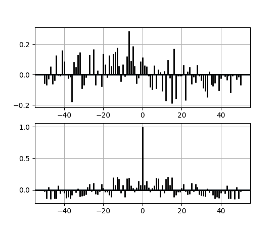
xcorris top graph, andacorris bottom graph.(Source code, png, pdf)
Note
In addition to the above described arguments, this function can take a data keyword argument. If such a data argument is given, the following arguments are replaced by data[<arg>]:
- All arguments with the following names: ‘x’.
-
matplotlib.pyplot.angle_spectrum(x, Fs=None, Fc=None, window=None, pad_to=None, sides=None, hold=None, data=None, **kwargs)¶ Plot the angle spectrum.
Call signature:
angle_spectrum(x, Fs=2, Fc=0,  window=mlab.window_hanning,
               pad_to=None, sides='default', **kwargs)
Compute the angle spectrum (wrapped phase spectrum) of x. Data is padded to a length of pad_to and the windowing function window is applied to the signal.
Parameters: x : 1-D array or sequence
Array or sequence containing the data
Fs : scalar
The sampling frequency (samples per time unit). It is used to calculate the Fourier frequencies, freqs, in cycles per time unit. The default value is 2.
window : callable or ndarray
A function or a vector of length NFFT. To create window vectors see
window_hanning(),window_none(),numpy.blackman(),numpy.hamming(),numpy.bartlett(),scipy.signal(),scipy.signal.get_window(), etc. The default iswindow_hanning(). If a function is passed as the argument, it must take a data segment as an argument and return the windowed version of the segment.sides : [ ‘default’ | ‘onesided’ | ‘twosided’ ]
Specifies which sides of the spectrum to return. Default gives the default behavior, which returns one-sided for real data and both for complex data. ‘onesided’ forces the return of a one-sided spectrum, while ‘twosided’ forces two-sided.
pad_to : integer
The number of points to which the data segment is padded when performing the FFT. While not increasing the actual resolution of the spectrum (the minimum distance between resolvable peaks), this can give more points in the plot, allowing for more detail. This corresponds to the n parameter in the call to fft(). The default is None, which sets pad_to equal to the length of the input signal (i.e. no padding).
Fc : integer
The center frequency of x (defaults to 0), which offsets the x extents of the plot to reflect the frequency range used when a signal is acquired and then filtered and downsampled to baseband.
**kwargs :
Keyword arguments control the
Line2Dproperties:Property Description agg_filterunknown alphafloat (0.0 transparent through 1.0 opaque) animated[True | False] antialiasedor aa[True | False] axesan Axesinstanceclip_boxa matplotlib.transforms.Bboxinstanceclip_on[True | False] clip_path[ ( Path,Transform) |Patch| None ]coloror cany matplotlib color containsa callable function dash_capstyle[‘butt’ | ‘round’ | ‘projecting’] dash_joinstyle[‘miter’ | ‘round’ | ‘bevel’] dashessequence of on/off ink in points drawstyle[‘default’ | ‘steps’ | ‘steps-pre’ | ‘steps-mid’ | ‘steps-post’] figurea matplotlib.figure.Figureinstancefillstyle[‘full’ | ‘left’ | ‘right’ | ‘bottom’ | ‘top’ | ‘none’] gidan id string labelstring or anything printable with ‘%s’ conversion. linestyleor ls[‘solid’ | ‘dashed’, ‘dashdot’, ‘dotted’ | (offset, on-off-dash-seq) | '-'|'--'|'-.'|':'|'None'|' '|'']linewidthor lwfloat value in points markerA valid marker stylemarkeredgecoloror mecany matplotlib color markeredgewidthor mewfloat value in points markerfacecoloror mfcany matplotlib color markerfacecoloraltor mfcaltany matplotlib color markersizeor msfloat markevery[None | int | length-2 tuple of int | slice | list/array of int | float | length-2 tuple of float] path_effectsunknown pickerfloat distance in points or callable pick function fn(artist, event)pickradiusfloat distance in points rasterized[True | False | None] sketch_paramsunknown snapunknown solid_capstyle[‘butt’ | ‘round’ | ‘projecting’] solid_joinstyle[‘miter’ | ‘round’ | ‘bevel’] transforma matplotlib.transforms.Transforminstanceurla url string visible[True | False] xdata1D array ydata1D array zorderany number Returns: spectrum : 1-D array
The values for the angle spectrum in radians (real valued)
freqs : 1-D array
The frequencies corresponding to the elements in spectrum
line : a
Line2DinstanceThe line created by this function
See also
magnitude_spectrum()angle_spectrum()plots the magnitudes of the corresponding frequencies.phase_spectrum()phase_spectrum()plots the unwrapped version of this function.specgram()specgram()can plot the angle spectrum of segments within the signal in a colormap.- In addition to the above described arguments, this function can take a data keyword argument. If such a data argument is given, the following arguments are replaced by data[<arg>]: * All arguments with the following names: ‘x’.
Examples
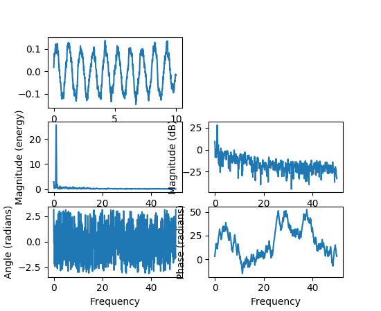
(Source code, png, pdf)
-
matplotlib.pyplot.annotate(*args, **kwargs)¶ Annotate the point
xywith texts.Additional kwargs are passed to
Text.Parameters: s : str
The text of the annotation
xy : iterable
Length 2 sequence specifying the (x,y) point to annotate
xytext : iterable, optional
Length 2 sequence specifying the (x,y) to place the text at. If None, defaults to
xy.xycoords : str, Artist, Transform, callable or tuple, optional
The coordinate system that
xyis given in.For a
strthe allowed values are:Property Description ‘figure points’ points from the lower left of the figure ‘figure pixels’ pixels from the lower left of the figure ‘figure fraction’ fraction of figure from lower left ‘axes points’ points from lower left corner of axes ‘axes pixels’ pixels from lower left corner of axes ‘axes fraction’ fraction of axes from lower left ‘data’ use the coordinate system of the object being annotated (default) ‘polar’ (theta,r) if not native ‘data’ coordinates If a
Artistobject is passed in the units are fraction if it’s bounding box.If a
Transformobject is passed in use that to transformxyto screen coordinatesIf a callable it must take a
RendererBaseobject as input and return aTransformorBboxobjectIf a
tuplemust be length 2 tuple of str,Artist,Transformor callable objects. The first transform is used for the x coordinate and the second for y.See Advanced Annotation for more details.
Defaults to
'data'textcoords : str,
Artist,Transform, callable or tuple, optionalThe coordinate system that
xytextis given, which may be different than the coordinate system used forxy.All
xycoordsvalues are valid as well as the following strings:Property Description ‘offset points’ offset (in points) from the xy value ‘offset pixels’ offset (in pixels) from the xy value defaults to the input of
xycoordsarrowprops : dict, optional
If not None, properties used to draw a
FancyArrowPatcharrow betweenxyandxytext.If
arrowpropsdoes not contain the key'arrowstyle'the allowed keys are:Key Description width the width of the arrow in points headwidth the width of the base of the arrow head in points headlength the length of the arrow head in points shrink fraction of total length to ‘shrink’ from both ends ? any key to matplotlib.patches.FancyArrowPatchIf the
arrowpropscontains the key'arrowstyle'the above keys are forbidden. The allowed values of'arrowstyle'are:Name Attrs '-'None '->'head_length=0.4,head_width=0.2 '-['widthB=1.0,lengthB=0.2,angleB=None '|-|'widthA=1.0,widthB=1.0 '-|>'head_length=0.4,head_width=0.2 '<-'head_length=0.4,head_width=0.2 '<->'head_length=0.4,head_width=0.2 '<|-'head_length=0.4,head_width=0.2 '<|-|>'head_length=0.4,head_width=0.2 'fancy'head_length=0.4,head_width=0.4,tail_width=0.4 'simple'head_length=0.5,head_width=0.5,tail_width=0.2 'wedge'tail_width=0.3,shrink_factor=0.5 Valid keys for
FancyArrowPatchare:Key Description arrowstyle the arrow style connectionstyle the connection style relpos default is (0.5, 0.5) patchA default is bounding box of the text patchB default is None shrinkA default is 2 points shrinkB default is 2 points mutation_scale default is text size (in points) mutation_aspect default is 1. ? any key for matplotlib.patches.PathPatchDefaults to None
annotation_clip : bool, optional
Controls the visibility of the annotation when it goes outside the axes area.
If
True, the annotation will only be drawn when thexyis inside the axes. IfFalse, the annotation will always be drawn regardless of its position.The default is
None, which behave asTrueonly if xycoords is “data”.Returns: Annotation
-
matplotlib.pyplot.arrow(x, y, dx, dy, hold=None, **kwargs)¶ Add an arrow to the axes.
Draws arrow on specified axis from (
x,y) to (x+dx,y+dy). Uses FancyArrow patch to construct the arrow.Parameters: x : float
X-coordinate of the arrow base
y : float
Y-coordinate of the arrow base
dx : float
Length of arrow along x-coordinate
dy : float
Length of arrow along y-coordinate
Returns: a : FancyArrow
patches.FancyArrow object
Other Parameters: Optional kwargs (inherited from FancyArrow patch) control the arrow
construction and properties:
Constructor arguments
- width: float (default: 0.001)
width of full arrow tail
- length_includes_head: [True | False] (default: False)
True if head is to be counted in calculating the length.
- head_width: float or None (default: 3*width)
total width of the full arrow head
- head_length: float or None (default: 1.5 * head_width)
length of arrow head
- shape: [‘full’, ‘left’, ‘right’] (default: ‘full’)
draw the left-half, right-half, or full arrow
- overhang: float (default: 0)
fraction that the arrow is swept back (0 overhang means triangular shape). Can be negative or greater than one.
- head_starts_at_zero: [True | False] (default: False)
if True, the head starts being drawn at coordinate 0 instead of ending at coordinate 0.
Other valid kwargs (inherited from :class:`Patch`) are:
Property Description agg_filterunknown alphafloat or None animated[True | False] antialiasedor aa[True | False] or None for default axesan Axesinstancecapstyle[‘butt’ | ‘round’ | ‘projecting’] clip_boxa matplotlib.transforms.Bboxinstanceclip_on[True | False] clip_path[ ( Path,Transform) |Patch| None ]colormatplotlib color spec containsa callable function edgecoloror ecmpl color spec, None, ‘none’, or ‘auto’ facecoloror fcmpl color spec, or None for default, or ‘none’ for no color figurea matplotlib.figure.Figureinstancefill[True | False] gidan id string hatch[‘/’ | ‘\’ | ‘|’ | ‘-‘ | ‘+’ | ‘x’ | ‘o’ | ‘O’ | ‘.’ | ‘*’] joinstyle[‘miter’ | ‘round’ | ‘bevel’] labelstring or anything printable with ‘%s’ conversion. linestyleor ls[‘solid’ | ‘dashed’, ‘dashdot’, ‘dotted’ | (offset, on-off-dash-seq) | '-'|'--'|'-.'|':'|'None'|' '|'']linewidthor lwfloat or None for default path_effectsunknown picker[None|float|boolean|callable] rasterized[True | False | None] sketch_paramsunknown snapunknown transformTransforminstanceurla url string visible[True | False] zorderany number Notes
The resulting arrow is affected by the axes aspect ratio and limits. This may produce an arrow whose head is not square with its stem. To create an arrow whose head is square with its stem, use
annotate()for example:ax.annotate("", xy=(0.5, 0.5), xytext=(0, 0), arrowprops=dict(arrowstyle="->"))
Examples
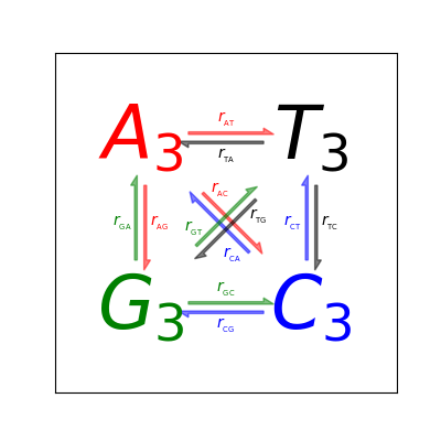
(Source code, png, pdf)
-
matplotlib.pyplot.autoscale(enable=True, axis='both', tight=None)¶ Autoscale the axis view to the data (toggle).
Convenience method for simple axis view autoscaling. It turns autoscaling on or off, and then, if autoscaling for either axis is on, it performs the autoscaling on the specified axis or axes.
- enable: [True | False | None]
- True (default) turns autoscaling on, False turns it off. None leaves the autoscaling state unchanged.
- axis: [‘x’ | ‘y’ | ‘both’]
- which axis to operate on; default is ‘both’
- tight: [True | False | None]
- If True, set view limits to data limits; if False, let the locator and margins expand the view limits; if None, use tight scaling if the only artist is an image, otherwise treat tight as False. The tight setting is retained for future autoscaling until it is explicitly changed.
Returns None.
-
matplotlib.pyplot.autumn()¶ set the default colormap to autumn and apply to current image if any. See help(colormaps) for more information
-
matplotlib.pyplot.axes(*args, **kwargs)¶ Add an axes to the figure.
The axes is added at position rect specified by:
axes()by itself creates a default fullsubplot(111)window axis.axes(rect, facecolor='w')where rect = [left, bottom, width, height] in normalized (0, 1) units. facecolor is the background color for the axis, default white.axes(h)where h is an axes instance makes h the current axis. AnAxesinstance is returned.
kwarg Accepts Description facecolor color the axes background color frameon [True|False] display the frame? sharex otherax current axes shares xaxis attribute with otherax sharey otherax current axes shares yaxis attribute with otherax polar [True|False] use a polar axes? aspect [str | num] [‘equal’, ‘auto’] or a number. If a number the ratio of x-unit/y-unit in screen-space. Also see set_aspect().Examples:
examples/pylab_examples/axes_demo.pyplaces custom axes.examples/pylab_examples/shared_axis_demo.pyuses sharex and sharey.
-
matplotlib.pyplot.axhline(y=0, xmin=0, xmax=1, hold=None, **kwargs)¶ Add a horizontal line across the axis.
Parameters: y : scalar, optional, default: 0
y position in data coordinates of the horizontal line.
xmin : scalar, optional, default: 0
Should be between 0 and 1, 0 being the far left of the plot, 1 the far right of the plot.
xmax : scalar, optional, default: 1
Should be between 0 and 1, 0 being the far left of the plot, 1 the far right of the plot.
Returns: See also
axhspan- for example plot and source code
Notes
kwargs are passed to
Line2Dand can be used to control the line properties.Examples
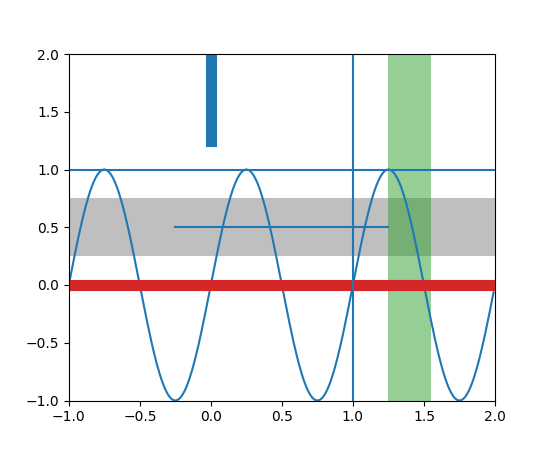
draw a thick red hline at ‘y’ = 0 that spans the xrange:
>>> axhline(linewidth=4, color='r')
draw a default hline at ‘y’ = 1 that spans the xrange:
>>> axhline(y=1)
draw a default hline at ‘y’ = .5 that spans the middle half of the xrange:
>>> axhline(y=.5, xmin=0.25, xmax=0.75)
Valid kwargs are
Line2Dproperties, with the exception of ‘transform’:Property Description agg_filterunknown alphafloat (0.0 transparent through 1.0 opaque) animated[True | False] antialiasedor aa[True | False] axesan Axesinstanceclip_boxa matplotlib.transforms.Bboxinstanceclip_on[True | False] clip_path[ ( Path,Transform) |Patch| None ]coloror cany matplotlib color containsa callable function dash_capstyle[‘butt’ | ‘round’ | ‘projecting’] dash_joinstyle[‘miter’ | ‘round’ | ‘bevel’] dashessequence of on/off ink in points drawstyle[‘default’ | ‘steps’ | ‘steps-pre’ | ‘steps-mid’ | ‘steps-post’] figurea matplotlib.figure.Figureinstancefillstyle[‘full’ | ‘left’ | ‘right’ | ‘bottom’ | ‘top’ | ‘none’] gidan id string labelstring or anything printable with ‘%s’ conversion. linestyleor ls[‘solid’ | ‘dashed’, ‘dashdot’, ‘dotted’ | (offset, on-off-dash-seq) | '-'|'--'|'-.'|':'|'None'|' '|'']linewidthor lwfloat value in points markerA valid marker stylemarkeredgecoloror mecany matplotlib color markeredgewidthor mewfloat value in points markerfacecoloror mfcany matplotlib color markerfacecoloraltor mfcaltany matplotlib color markersizeor msfloat markevery[None | int | length-2 tuple of int | slice | list/array of int | float | length-2 tuple of float] path_effectsunknown pickerfloat distance in points or callable pick function fn(artist, event)pickradiusfloat distance in points rasterized[True | False | None] sketch_paramsunknown snapunknown solid_capstyle[‘butt’ | ‘round’ | ‘projecting’] solid_joinstyle[‘miter’ | ‘round’ | ‘bevel’] transforma matplotlib.transforms.Transforminstanceurla url string visible[True | False] xdata1D array ydata1D array zorderany number
-
matplotlib.pyplot.axhspan(ymin, ymax, xmin=0, xmax=1, hold=None, **kwargs)¶ Add a horizontal span (rectangle) across the axis.
Draw a horizontal span (rectangle) from ymin to ymax. With the default values of xmin = 0 and xmax = 1, this always spans the xrange, regardless of the xlim settings, even if you change them, e.g., with the
set_xlim()command. That is, the horizontal extent is in axes coords: 0=left, 0.5=middle, 1.0=right but the y location is in data coordinates.Parameters: ymin : float
Lower limit of the horizontal span in data units.
ymax : float
Upper limit of the horizontal span in data units.
xmin : float, optional, default: 0
Lower limit of the vertical span in axes (relative 0-1) units.
xmax : float, optional, default: 1
Upper limit of the vertical span in axes (relative 0-1) units.
Returns: Polygon :
PolygonOther Parameters: kwargs :
Polygonproperties.Property Description agg_filterunknown alphafloat or None animated[True | False] antialiasedor aa[True | False] or None for default axesan Axesinstancecapstyle[‘butt’ | ‘round’ | ‘projecting’] clip_boxa matplotlib.transforms.Bboxinstanceclip_on[True | False] clip_path[ ( Path,Transform) |Patch| None ]colormatplotlib color spec containsa callable function edgecoloror ecmpl color spec, None, ‘none’, or ‘auto’ facecoloror fcmpl color spec, or None for default, or ‘none’ for no color figurea matplotlib.figure.Figureinstancefill[True | False] gidan id string hatch[‘/’ | ‘\’ | ‘|’ | ‘-‘ | ‘+’ | ‘x’ | ‘o’ | ‘O’ | ‘.’ | ‘*’] joinstyle[‘miter’ | ‘round’ | ‘bevel’] labelstring or anything printable with ‘%s’ conversion. linestyleor ls[‘solid’ | ‘dashed’, ‘dashdot’, ‘dotted’ | (offset, on-off-dash-seq) | '-'|'--'|'-.'|':'|'None'|' '|'']linewidthor lwfloat or None for default path_effectsunknown picker[None|float|boolean|callable] rasterized[True | False | None] sketch_paramsunknown snapunknown transformTransforminstanceurla url string visible[True | False] zorderany number See also
axvspan- Add a vertical span (rectangle) across the axes.
Examples
(Source code, png, pdf)
-
matplotlib.pyplot.axis(*v, **kwargs)¶ Convenience method to get or set axis properties.
Calling with no arguments:
>>> axis()
returns the current axes limits
[xmin, xmax, ymin, ymax].:>>> axis(v)
sets the min and max of the x and y axes, with
v = [xmin, xmax, ymin, ymax].:>>> axis('off')
turns off the axis lines and labels.:
>>> axis('equal')
changes limits of x or y axis so that equal increments of x and y have the same length; a circle is circular.:
>>> axis('scaled')
achieves the same result by changing the dimensions of the plot box instead of the axis data limits.:
>>> axis('tight')
changes x and y axis limits such that all data is shown. If all data is already shown, it will move it to the center of the figure without modifying (xmax - xmin) or (ymax - ymin). Note this is slightly different than in MATLAB.:
>>> axis('image')
is ‘scaled’ with the axis limits equal to the data limits.:
>>> axis('auto')
and:
>>> axis('normal')
are deprecated. They restore default behavior; axis limits are automatically scaled to make the data fit comfortably within the plot box.
if
len(*v)==0, you can pass in xmin, xmax, ymin, ymax as kwargs selectively to alter just those limits without changing the others.>>> axis('square')
changes the limit ranges (xmax-xmin) and (ymax-ymin) of the x and y axes to be the same, and have the same scaling, resulting in a square plot.
The xmin, xmax, ymin, ymax tuple is returned
-
matplotlib.pyplot.axvline(x=0, ymin=0, ymax=1, hold=None, **kwargs)¶ Add a vertical line across the axes.
Parameters: x : scalar, optional, default: 0
x position in data coordinates of the vertical line.
ymin : scalar, optional, default: 0
Should be between 0 and 1, 0 being the bottom of the plot, 1 the top of the plot.
ymax : scalar, optional, default: 1
Should be between 0 and 1, 0 being the bottom of the plot, 1 the top of the plot.
Returns: See also
axhspan- for example plot and source code
Examples
draw a thick red vline at x = 0 that spans the yrange:
>>> axvline(linewidth=4, color='r')
draw a default vline at x = 1 that spans the yrange:
>>> axvline(x=1)
draw a default vline at x = .5 that spans the middle half of the yrange:
>>> axvline(x=.5, ymin=0.25, ymax=0.75)
Valid kwargs are
Line2Dproperties, with the exception of ‘transform’:Property Description agg_filterunknown alphafloat (0.0 transparent through 1.0 opaque) animated[True | False] antialiasedor aa[True | False] axesan Axesinstanceclip_boxa matplotlib.transforms.Bboxinstanceclip_on[True | False] clip_path[ ( Path,Transform) |Patch| None ]coloror cany matplotlib color containsa callable function dash_capstyle[‘butt’ | ‘round’ | ‘projecting’] dash_joinstyle[‘miter’ | ‘round’ | ‘bevel’] dashessequence of on/off ink in points drawstyle[‘default’ | ‘steps’ | ‘steps-pre’ | ‘steps-mid’ | ‘steps-post’] figurea matplotlib.figure.Figureinstancefillstyle[‘full’ | ‘left’ | ‘right’ | ‘bottom’ | ‘top’ | ‘none’] gidan id string labelstring or anything printable with ‘%s’ conversion. linestyleor ls[‘solid’ | ‘dashed’, ‘dashdot’, ‘dotted’ | (offset, on-off-dash-seq) | '-'|'--'|'-.'|':'|'None'|' '|'']linewidthor lwfloat value in points markerA valid marker stylemarkeredgecoloror mecany matplotlib color markeredgewidthor mewfloat value in points markerfacecoloror mfcany matplotlib color markerfacecoloraltor mfcaltany matplotlib color markersizeor msfloat markevery[None | int | length-2 tuple of int | slice | list/array of int | float | length-2 tuple of float] path_effectsunknown pickerfloat distance in points or callable pick function fn(artist, event)pickradiusfloat distance in points rasterized[True | False | None] sketch_paramsunknown snapunknown solid_capstyle[‘butt’ | ‘round’ | ‘projecting’] solid_joinstyle[‘miter’ | ‘round’ | ‘bevel’] transforma matplotlib.transforms.Transforminstanceurla url string visible[True | False] xdata1D array ydata1D array zorderany number
-
matplotlib.pyplot.axvspan(xmin, xmax, ymin=0, ymax=1, hold=None, **kwargs)¶ Add a vertical span (rectangle) across the axes.
Draw a vertical span (rectangle) from
xmintoxmax. With the default values ofymin= 0 andymax= 1. This always spans the yrange, regardless of the ylim settings, even if you change them, e.g., with theset_ylim()command. That is, the vertical extent is in axes coords: 0=bottom, 0.5=middle, 1.0=top but the y location is in data coordinates.Parameters: xmin : scalar
Number indicating the first X-axis coordinate of the vertical span rectangle in data units.
xmax : scalar
Number indicating the second X-axis coordinate of the vertical span rectangle in data units.
ymin : scalar, optional
Number indicating the first Y-axis coordinate of the vertical span rectangle in relative Y-axis units (0-1). Default to 0.
ymax : scalar, optional
Number indicating the second Y-axis coordinate of the vertical span rectangle in relative Y-axis units (0-1). Default to 1.
Returns: rectangle : matplotlib.patches.Polygon
Vertical span (rectangle) from (xmin, ymin) to (xmax, ymax).
Other Parameters: **kwargs
Optional parameters are properties of the class matplotlib.patches.Polygon.
Examples
Draw a vertical, green, translucent rectangle from x = 1.25 to x = 1.55 that spans the yrange of the axes.
>>> axvspan(1.25, 1.55, facecolor='g', alpha=0.5)
-
matplotlib.pyplot.bar(left, height, width=0.8, bottom=None, hold=None, data=None, **kwargs)¶ Make a bar plot.
Make a bar plot with rectangles bounded by:
left,left+width,bottom,bottom+height- (left, right, bottom and top edges)
Parameters: left : sequence of scalars
the x coordinates of the left sides of the bars
height : sequence of scalars
the heights of the bars
width : scalar or array-like, optional
the width(s) of the bars default: 0.8
bottom : scalar or array-like, optional
the y coordinate(s) of the bars default: None
color : scalar or array-like, optional
the colors of the bar faces
edgecolor : scalar or array-like, optional
the colors of the bar edges
linewidth : scalar or array-like, optional
width of bar edge(s). If None, use default linewidth; If 0, don’t draw edges. default: None
tick_label : string or array-like, optional
the tick labels of the bars default: None
xerr : scalar or array-like, optional
if not None, will be used to generate errorbar(s) on the bar chart default: None
yerr : scalar or array-like, optional
if not None, will be used to generate errorbar(s) on the bar chart default: None
ecolor : scalar or array-like, optional
specifies the color of errorbar(s) default: None
capsize : scalar, optional
determines the length in points of the error bar caps default: None, which will take the value from the
errorbar.capsizercParam.error_kw : dict, optional
dictionary of kwargs to be passed to errorbar method. ecolor and capsize may be specified here rather than as independent kwargs.
align : {‘center’, ‘edge’}, optional
If ‘edge’, aligns bars by their left edges (for vertical bars) and by their bottom edges (for horizontal bars). If ‘center’, interpret the
leftargument as the coordinates of the centers of the bars. To align on the align bars on the right edge pass a negativewidth.orientation : {‘vertical’, ‘horizontal’}, optional
The orientation of the bars.
log : boolean, optional
If true, sets the axis to be log scale. default: False
Returns: bars : matplotlib.container.BarContainer
Container with all of the bars + errorbars
See also
barh- Plot a horizontal bar plot.
Notes
The optional arguments
color,edgecolor,linewidth,xerr, andyerrcan be either scalars or sequences of length equal to the number of bars. This enables you to use bar as the basis for stacked bar charts, or candlestick plots. Detail:xerrandyerrare passed directly toerrorbar(), so they can also have shape 2xN for independent specification of lower and upper errors.Other optional kwargs:
Property Description agg_filterunknown alphafloat or None animated[True | False] antialiasedor aa[True | False] or None for default axesan Axesinstancecapstyle[‘butt’ | ‘round’ | ‘projecting’] clip_boxa matplotlib.transforms.Bboxinstanceclip_on[True | False] clip_path[ ( Path,Transform) |Patch| None ]colormatplotlib color spec containsa callable function edgecoloror ecmpl color spec, None, ‘none’, or ‘auto’ facecoloror fcmpl color spec, or None for default, or ‘none’ for no color figurea matplotlib.figure.Figureinstancefill[True | False] gidan id string hatch[‘/’ | ‘\’ | ‘|’ | ‘-‘ | ‘+’ | ‘x’ | ‘o’ | ‘O’ | ‘.’ | ‘*’] joinstyle[‘miter’ | ‘round’ | ‘bevel’] labelstring or anything printable with ‘%s’ conversion. linestyleor ls[‘solid’ | ‘dashed’, ‘dashdot’, ‘dotted’ | (offset, on-off-dash-seq) | '-'|'--'|'-.'|':'|'None'|' '|'']linewidthor lwfloat or None for default path_effectsunknown picker[None|float|boolean|callable] rasterized[True | False | None] sketch_paramsunknown snapunknown transformTransforminstanceurla url string visible[True | False] zorderany number Examples
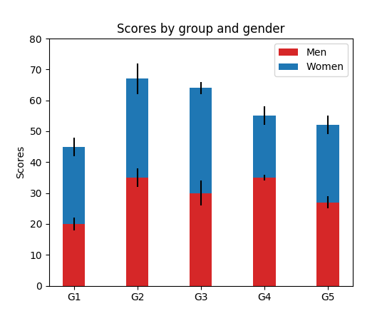
Example: A stacked bar chart.
(Source code, png, pdf)
Note
In addition to the above described arguments, this function can take a data keyword argument. If such a data argument is given, the following arguments are replaced by data[<arg>]:
- All arguments with the following names: ‘bottom’, ‘color’, ‘ecolor’, ‘edgecolor’, ‘height’, ‘left’, ‘linewidth’, ‘tick_label’, ‘width’, ‘xerr’, ‘yerr’.
-
matplotlib.pyplot.barbs(*args, **kw)¶ Plot a 2-D field of barbs.
Call signatures:
barb(U, V, **kw)
barb(U, V, C, **kw)
barb(X, Y, U, V, **kw)
barb(X, Y, U, V, C, **kw)
Arguments:
- X, Y:
- The x and y coordinates of the barb locations (default is head of barb; see pivot kwarg)
- U, V:
- Give the x and y components of the barb shaft
- C:
- An optional array used to map colors to the barbs
All arguments may be 1-D or 2-D arrays or sequences. If X and Y are absent, they will be generated as a uniform grid. If U and V are 2-D arrays but X and Y are 1-D, and if
len(X)andlen(Y)match the column and row dimensions of U, then X and Y will be expanded withnumpy.meshgrid().U, V, C may be masked arrays, but masked X, Y are not supported at present.
Keyword arguments:
- length:
- Length of the barb in points; the other parts of the barb are scaled against this. Default is 9
- pivot: [ ‘tip’ | ‘middle’ ]
- The part of the arrow that is at the grid point; the arrow rotates about this point, hence the name pivot. Default is ‘tip’
- barbcolor: [ color | color sequence ]
- Specifies the color all parts of the barb except any flags. This parameter is analagous to the edgecolor parameter for polygons, which can be used instead. However this parameter will override facecolor.
- flagcolor: [ color | color sequence ]
- Specifies the color of any flags on the barb. This parameter is analagous to the facecolor parameter for polygons, which can be used instead. However this parameter will override facecolor. If this is not set (and C has not either) then flagcolor will be set to match barbcolor so that the barb has a uniform color. If C has been set, flagcolor has no effect.
- sizes:
A dictionary of coefficients specifying the ratio of a given feature to the length of the barb. Only those values one wishes to override need to be included. These features include:
- ‘spacing’ - space between features (flags, full/half barbs)
- ‘height’ - height (distance from shaft to top) of a flag or full barb
- ‘width’ - width of a flag, twice the width of a full barb
- ‘emptybarb’ - radius of the circle used for low magnitudes
- fill_empty:
- A flag on whether the empty barbs (circles) that are drawn should be filled with the flag color. If they are not filled, they will be drawn such that no color is applied to the center. Default is False
- rounding:
- A flag to indicate whether the vector magnitude should be rounded when allocating barb components. If True, the magnitude is rounded to the nearest multiple of the half-barb increment. If False, the magnitude is simply truncated to the next lowest multiple. Default is True
- barb_increments:
A dictionary of increments specifying values to associate with different parts of the barb. Only those values one wishes to override need to be included.
- ‘half’ - half barbs (Default is 5)
- ‘full’ - full barbs (Default is 10)
- ‘flag’ - flags (default is 50)
- flip_barb:
- Either a single boolean flag or an array of booleans. Single boolean indicates whether the lines and flags should point opposite to normal for all barbs. An array (which should be the same size as the other data arrays) indicates whether to flip for each individual barb. Normal behavior is for the barbs and lines to point right (comes from wind barbs having these features point towards low pressure in the Northern Hemisphere.) Default is False
Barbs are traditionally used in meteorology as a way to plot the speed and direction of wind observations, but can technically be used to plot any two dimensional vector quantity. As opposed to arrows, which give vector magnitude by the length of the arrow, the barbs give more quantitative information about the vector magnitude by putting slanted lines or a triangle for various increments in magnitude, as show schematically below:
:     /\    \
:    /  \    \
:   /    \    \    \
:  /      \    \    \
: ------------------------------
The largest increment is given by a triangle (or “flag”). After those come full lines (barbs). The smallest increment is a half line. There is only, of course, ever at most 1 half line. If the magnitude is small and only needs a single half-line and no full lines or triangles, the half-line is offset from the end of the barb so that it can be easily distinguished from barbs with a single full line. The magnitude for the barb shown above would nominally be 65, using the standard increments of 50, 10, and 5.
linewidths and edgecolors can be used to customize the barb. Additional
PolyCollectionkeyword arguments:Property Description agg_filterunknown alphafloat or None animated[True | False] antialiasedor antialiasedsBoolean or sequence of booleans arrayunknown axesan Axesinstanceclima length 2 sequence of floats clip_boxa matplotlib.transforms.Bboxinstanceclip_on[True | False] clip_path[ ( Path,Transform) |Patch| None ]cmapa colormap or registered colormap name colormatplotlib color arg or sequence of rgba tuples containsa callable function edgecoloror edgecolorsmatplotlib color spec or sequence of specs facecoloror facecolorsmatplotlib color spec or sequence of specs figurea matplotlib.figure.Figureinstancegidan id string hatch[ ‘/’ | ‘\’ | ‘|’ | ‘-‘ | ‘+’ | ‘x’ | ‘o’ | ‘O’ | ‘.’ | ‘*’ ] labelstring or anything printable with ‘%s’ conversion. linestyleor dashes or linestyles[‘solid’ | ‘dashed’, ‘dashdot’, ‘dotted’ | (offset, on-off-dash-seq) | '-'|'--'|'-.'|':'|'None'|' '|'']linewidthor linewidths or lwfloat or sequence of floats normunknown offset_positionunknown offsetsfloat or sequence of floats path_effectsunknown picker[None|float|boolean|callable] pickradiusunknown rasterized[True | False | None] sketch_paramsunknown snapunknown transformTransforminstanceurla url string urlsunknown visible[True | False] zorderany number Example:
Note
In addition to the above described arguments, this function can take a data keyword argument. If such a data argument is given, the following arguments are replaced by data[<arg>]:
- All positional and all keyword arguments.
-
matplotlib.pyplot.barh(bottom, width, height=0.8, left=None, hold=None, **kwargs)¶ Make a horizontal bar plot.
Make a horizontal bar plot with rectangles bounded by:
left,left+width,bottom,bottom+height- (left, right, bottom and top edges)
bottom,width,height, andleftcan be either scalars or sequencesParameters: bottom : scalar or array-like
the y coordinate(s) of the bars
width : scalar or array-like
the width(s) of the bars
height : sequence of scalars, optional, default: 0.8
the heights of the bars
left : sequence of scalars
the x coordinates of the left sides of the bars
Returns: matplotlib.patches.Rectangleinstances.Other Parameters: color : scalar or array-like, optional
the colors of the bars
edgecolor : scalar or array-like, optional
the colors of the bar edges
linewidth : scalar or array-like, optional, default: None
width of bar edge(s). If None, use default linewidth; If 0, don’t draw edges.
tick_label : string or array-like, optional, default: None
the tick labels of the bars
xerr : scalar or array-like, optional, default: None
if not None, will be used to generate errorbar(s) on the bar chart
yerr : scalar or array-like, optional, default: None
if not None, will be used to generate errorbar(s) on the bar chart
ecolor : scalar or array-like, optional, default: None
specifies the color of errorbar(s)
capsize : scalar, optional
determines the length in points of the error bar caps default: None, which will take the value from the
errorbar.capsizercParam.error_kw :
dictionary of kwargs to be passed to errorbar method.
ecolorandcapsizemay be specified here rather than as independent kwargs.align : {‘center’, ‘edge’}, optional
If ‘edge’, aligns bars by their left edges (for vertical bars) and by their bottom edges (for horizontal bars). If ‘center’, interpret the
bottomargument as the coordinates of the centers of the bars. To align on the align bars on the top edge pass a negative ‘height’.log : boolean, optional, default: False
If true, sets the axis to be log scale
See also
bar- Plot a vertical bar plot.
Notes
The optional arguments
color,edgecolor,linewidth,xerr, andyerrcan be either scalars or sequences of length equal to the number of bars. This enables you to use bar as the basis for stacked bar charts, or candlestick plots. Detail:xerrandyerrare passed directly toerrorbar(), so they can also have shape 2xN for independent specification of lower and upper errors.Other optional kwargs:
Property Description agg_filterunknown alphafloat or None animated[True | False] antialiasedor aa[True | False] or None for default axesan Axesinstancecapstyle[‘butt’ | ‘round’ | ‘projecting’] clip_boxa matplotlib.transforms.Bboxinstanceclip_on[True | False] clip_path[ ( Path,Transform) |Patch| None ]colormatplotlib color spec containsa callable function edgecoloror ecmpl color spec, None, ‘none’, or ‘auto’ facecoloror fcmpl color spec, or None for default, or ‘none’ for no color figurea matplotlib.figure.Figureinstancefill[True | False] gidan id string hatch[‘/’ | ‘\’ | ‘|’ | ‘-‘ | ‘+’ | ‘x’ | ‘o’ | ‘O’ | ‘.’ | ‘*’] joinstyle[‘miter’ | ‘round’ | ‘bevel’] labelstring or anything printable with ‘%s’ conversion. linestyleor ls[‘solid’ | ‘dashed’, ‘dashdot’, ‘dotted’ | (offset, on-off-dash-seq) | '-'|'--'|'-.'|':'|'None'|' '|'']linewidthor lwfloat or None for default path_effectsunknown picker[None|float|boolean|callable] rasterized[True | False | None] sketch_paramsunknown snapunknown transformTransforminstanceurla url string visible[True | False] zorderany number
-
matplotlib.pyplot.bone()¶ set the default colormap to bone and apply to current image if any. See help(colormaps) for more information
-
matplotlib.pyplot.box(on=None)¶ Turn the axes box on or off. on may be a boolean or a string, ‘on’ or ‘off’.
If on is None, toggle state.
-
matplotlib.pyplot.boxplot(x, notch=None, sym=None, vert=None, whis=None, positions=None, widths=None, patch_artist=None, bootstrap=None, usermedians=None, conf_intervals=None, meanline=None, showmeans=None, showcaps=None, showbox=None, showfliers=None, boxprops=None, labels=None, flierprops=None, medianprops=None, meanprops=None, capprops=None, whiskerprops=None, manage_xticks=True, autorange=False, zorder=None, hold=None, data=None)¶ Make a box and whisker plot.
Make a box and whisker plot for each column of
xor each vector in sequencex. The box extends from the lower to upper quartile values of the data, with a line at the median. The whiskers extend from the box to show the range of the data. Flier points are those past the end of the whiskers.Parameters: x : Array or a sequence of vectors.
The input data.
notch : bool, optional (False)
If
True, will produce a notched box plot. Otherwise, a rectangular boxplot is produced. The notches represent the confidence interval (CI) around the median. See the entry for thebootstrapparameter for information regarding how the locations of the notches are computed.Note
In cases where the values of the CI are less than the lower quartile or greater than the upper quartile, the notches will extend beyond the box, giving it a distinctive “flipped” appearance. This is expected behavior and consistent with other statistical visualization packages.
sym : str, optional
The default symbol for flier points. Enter an empty string (‘’) if you don’t want to show fliers. If
None, then the fliers default to ‘b+’ If you want more control use the flierprops kwarg.vert : bool, optional (True)
If
True(default), makes the boxes vertical. IfFalse, everything is drawn horizontally.whis : float, sequence, or string (default = 1.5)
As a float, determines the reach of the whiskers to the beyond the first and third quartiles. In other words, where IQR is the interquartile range (
Q3-Q1), the upper whisker will extend to last datum less thanQ3 + whis*IQR). Similarly, the lower whisker will extend to the first datum greater thanQ1 - whis*IQR. Beyond the whiskers, data are considered outliers and are plotted as individual points. Set this to an unreasonably high value to force the whiskers to show the min and max values. Alternatively, set this to an ascending sequence of percentile (e.g., [5, 95]) to set the whiskers at specific percentiles of the data. Finally,whiscan be the string'range'to force the whiskers to the min and max of the data.bootstrap : int, optional
Specifies whether to bootstrap the confidence intervals around the median for notched boxplots. If
bootstrapis None, no bootstrapping is performed, and notches are calculated using a Gaussian-based asymptotic approximation (see McGill, R., Tukey, J.W., and Larsen, W.A., 1978, and Kendall and Stuart, 1967). Otherwise, bootstrap specifies the number of times to bootstrap the median to determine its 95% confidence intervals. Values between 1000 and 10000 are recommended.usermedians : array-like, optional
An array or sequence whose first dimension (or length) is compatible with
x. This overrides the medians computed by matplotlib for each element ofusermediansthat is notNone. When an element ofusermediansis None, the median will be computed by matplotlib as normal.conf_intervals : array-like, optional
Array or sequence whose first dimension (or length) is compatible with
xand whose second dimension is 2. When the an element ofconf_intervalsis not None, the notch locations computed by matplotlib are overridden (providednotchisTrue). When an element ofconf_intervalsisNone, the notches are computed by the method specified by the other kwargs (e.g.,bootstrap).positions : array-like, optional
Sets the positions of the boxes. The ticks and limits are automatically set to match the positions. Defaults to
range(1, N+1)where N is the number of boxes to be drawn.widths : scalar or array-like
Sets the width of each box either with a scalar or a sequence. The default is 0.5, or
0.15*(distance between
extreme positions)
, if that is smaller.patch_artist : bool, optional (False)
If
Falseproduces boxes with the Line2D artist. Otherwise, boxes and drawn with Patch artists.labels : sequence, optional
Labels for each dataset. Length must be compatible with dimensions of
x.manage_xticks : bool, optional (True)
If the function should adjust the xlim and xtick locations.
autorange : bool, optional (False)
When
Trueand the data are distributed such that the 25th and 75th percentiles are equal,whisis set to'range'such that the whisker ends are at the minimum and maximum of the data.meanline : bool, optional (False)
If
True(andshowmeansisTrue), will try to render the mean as a line spanning the full width of the box according tomeanprops(see below). Not recommended ifshownotchesis also True. Otherwise, means will be shown as points.zorder : scalar, optional (None)
Sets the zorder of the boxplot.
Returns: result : dict
A dictionary mapping each component of the boxplot to a list of the
matplotlib.lines.Line2Dinstances created. That dictionary has the following keys (assuming vertical boxplots):boxes: the main body of the boxplot showing the quartiles and the median’s confidence intervals if enabled.medians: horizontal lines at the median of each box.whiskers: the vertical lines extending to the most extreme, non-outlier data points.caps: the horizontal lines at the ends of the whiskers.fliers: points representing data that extend beyond the whiskers (fliers).means: points or lines representing the means.
Other Parameters: showcaps : bool, optional (True)
Show the caps on the ends of whiskers.
showbox : bool, optional (True)
Show the central box.
showfliers : bool, optional (True)
Show the outliers beyond the caps.
showmeans : bool, optional (False)
Show the arithmetic means.
capprops : dict, optional (None)
Specifies the style of the caps.
boxprops : dict, optional (None)
Specifies the style of the box.
whiskerprops : dict, optional (None)
Specifies the style of the whiskers.
flierprops : dict, optional (None)
Specifies the style of the fliers.
medianprops : dict, optional (None)
Specifies the style of the median.
meanprops : dict, optional (None)
Specifies the style of the mean.
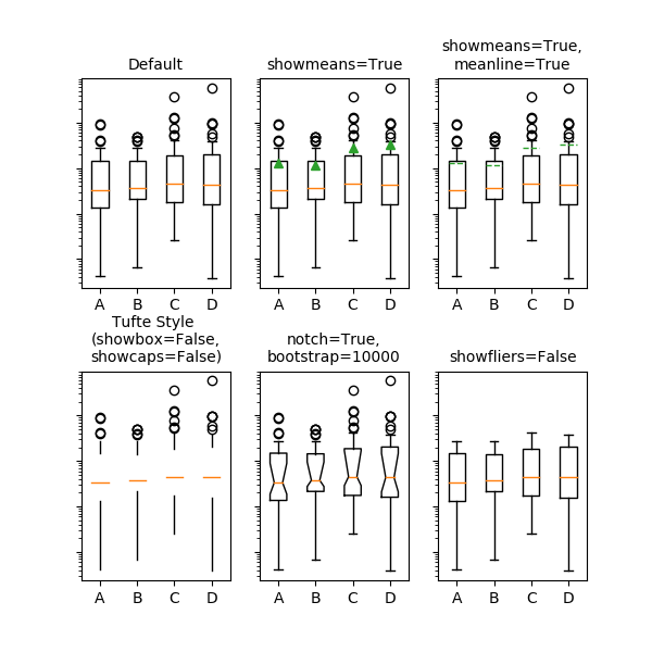
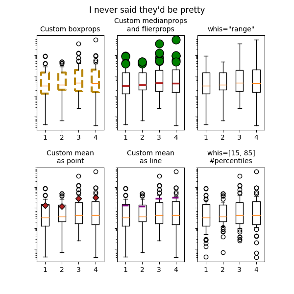
Examples
(Source code, png, pdf)
Note
In addition to the above described arguments, this function can take a data keyword argument. If such a data argument is given, the following arguments are replaced by data[<arg>]:
- All positional and all keyword arguments.
-
matplotlib.pyplot.broken_barh(xranges, yrange, hold=None, data=None, **kwargs)¶ Plot horizontal bars.
A collection of horizontal bars spanning yrange with a sequence of xranges.
Required arguments:
Argument Description xranges sequence of (xmin, xwidth) yrange sequence of (ymin, ywidth) kwargs are
matplotlib.collections.BrokenBarHCollectionproperties:Property Description agg_filterunknown alphafloat or None animated[True | False] antialiasedor antialiasedsBoolean or sequence of booleans arrayunknown axesan Axesinstanceclima length 2 sequence of floats clip_boxa matplotlib.transforms.Bboxinstanceclip_on[True | False] clip_path[ ( Path,Transform) |Patch| None ]cmapa colormap or registered colormap name colormatplotlib color arg or sequence of rgba tuples containsa callable function edgecoloror edgecolorsmatplotlib color spec or sequence of specs facecoloror facecolorsmatplotlib color spec or sequence of specs figurea matplotlib.figure.Figureinstancegidan id string hatch[ ‘/’ | ‘\’ | ‘|’ | ‘-‘ | ‘+’ | ‘x’ | ‘o’ | ‘O’ | ‘.’ | ‘*’ ] labelstring or anything printable with ‘%s’ conversion. linestyleor dashes or linestyles[‘solid’ | ‘dashed’, ‘dashdot’, ‘dotted’ | (offset, on-off-dash-seq) | '-'|'--'|'-.'|':'|'None'|' '|'']linewidthor linewidths or lwfloat or sequence of floats normunknown offset_positionunknown offsetsfloat or sequence of floats path_effectsunknown picker[None|float|boolean|callable] pickradiusunknown rasterized[True | False | None] sketch_paramsunknown snapunknown transformTransforminstanceurla url string urlsunknown visible[True | False] zorderany number these can either be a single argument, i.e.,:
facecolors = 'black'
or a sequence of arguments for the various bars, i.e.,:
facecolors = ('black', 'red', 'green')
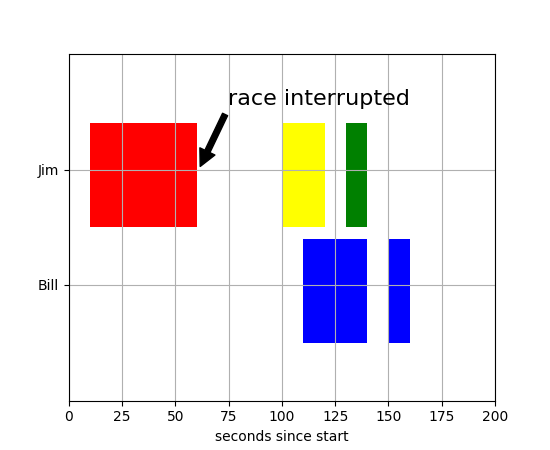
Example:
(Source code, png, pdf)
Note
In addition to the above described arguments, this function can take a data keyword argument. If such a data argument is given, the following arguments are replaced by data[<arg>]:
- All positional and all keyword arguments.
-
matplotlib.pyplot.cla()¶ Clear the current axes.
-
matplotlib.pyplot.clabel(CS, *args, **kwargs)¶ Label a contour plot.
Call signature:
clabel(cs, **kwargs)
Adds labels to line contours in cs, where cs is a
ContourSetobject returned by contour.clabel(cs, v, **kwargs)
only labels contours listed in v.
Optional keyword arguments:
- fontsize:
- size in points or relative size e.g., ‘smaller’, ‘x-large’
- colors:
- if None, the color of each label matches the color of the corresponding contour
- if one string color, e.g., colors = ‘r’ or colors = ‘red’, all labels will be plotted in this color
- if a tuple of matplotlib color args (string, float, rgb, etc), different labels will be plotted in different colors in the order specified
- inline:
- controls whether the underlying contour is removed or not. Default is True.
- inline_spacing:
- space in pixels to leave on each side of label when placing inline. Defaults to 5. This spacing will be exact for labels at locations where the contour is straight, less so for labels on curved contours.
- fmt:
- a format string for the label. Default is ‘%1.3f’
Alternatively, this can be a dictionary matching contour
levels with arbitrary strings to use for each contour level
(i.e., fmt[level]=string), or it can be any callable, such
as a
Formatterinstance, that returns a string when called with a numeric contour level. - manual:
if True, contour labels will be placed manually using mouse clicks. Click the first button near a contour to add a label, click the second button (or potentially both mouse buttons at once) to finish adding labels. The third button can be used to remove the last label added, but only if labels are not inline. Alternatively, the keyboard can be used to select label locations (enter to end label placement, delete or backspace act like the third mouse button, and any other key will select a label location).
manual can be an iterable object of x,y tuples. Contour labels will be created as if mouse is clicked at each x,y positions.
- rightside_up:
- if True (default), label rotations will always be plus or minus 90 degrees from level.
- use_clabeltext:
- if True (default is False), ClabelText class (instead of matplotlib.Text) is used to create labels. ClabelText recalculates rotation angles of texts during the drawing time, therefore this can be used if aspect of the axes changes.
-
matplotlib.pyplot.clf()¶ Clear the current figure.
-
matplotlib.pyplot.clim(vmin=None, vmax=None)¶ Set the color limits of the current image.
To apply clim to all axes images do:
clim(0, 0.5)
If either vmin or vmax is None, the image min/max respectively will be used for color scaling.
If you want to set the clim of multiple images, use, for example:
for im in gca().get_images():
    im.set_clim(0, 0.05)
-
matplotlib.pyplot.close(*args)¶ Close a figure window.
close()by itself closes the current figureclose(h)where h is aFigureinstance, closes that figureclose(num)closes figure number numclose(name)where name is a string, closes figure with that labelclose('all')closes all the figure windows
-
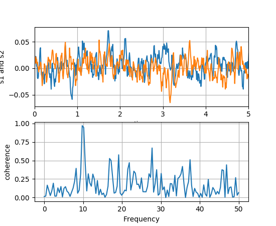
matplotlib.pyplot.cohere(x, y, NFFT=256, Fs=2, Fc=0, detrend=<function detrend_none>, window=<function window_hanning>, noverlap=0, pad_to=None, sides='default', scale_by_freq=None, hold=None, data=None, **kwargs)¶ Plot the coherence between x and y.
Plot the coherence between x and y. Coherence is the normalized cross spectral density:

Parameters: Fs : scalar
The sampling frequency (samples per time unit). It is used to calculate the Fourier frequencies, freqs, in cycles per time unit. The default value is 2.
window : callable or ndarray
A function or a vector of length NFFT. To create window vectors see
window_hanning(),window_none(),numpy.blackman(),numpy.hamming(),numpy.bartlett(),scipy.signal(),scipy.signal.get_window(), etc. The default iswindow_hanning(). If a function is passed as the argument, it must take a data segment as an argument and return the windowed version of the segment.sides : [ ‘default’ | ‘onesided’ | ‘twosided’ ]
Specifies which sides of the spectrum to return. Default gives the default behavior, which returns one-sided for real data and both for complex data. ‘onesided’ forces the return of a one-sided spectrum, while ‘twosided’ forces two-sided.
pad_to : integer
The number of points to which the data segment is padded when performing the FFT. This can be different from NFFT, which specifies the number of data points used. While not increasing the actual resolution of the spectrum (the minimum distance between resolvable peaks), this can give more points in the plot, allowing for more detail. This corresponds to the n parameter in the call to fft(). The default is None, which sets pad_to equal to NFFT
NFFT : integer
The number of data points used in each block for the FFT. A power 2 is most efficient. The default value is 256. This should NOT be used to get zero padding, or the scaling of the result will be incorrect. Use pad_to for this instead.
detrend : {‘default’, ‘constant’, ‘mean’, ‘linear’, ‘none’} or callable
The function applied to each segment before fft-ing, designed to remove the mean or linear trend. Unlike in MATLAB, where the detrend parameter is a vector, in matplotlib is it a function. The
pylabmodule definesdetrend_none(),detrend_mean(), anddetrend_linear(), but you can use a custom function as well. You can also use a string to choose one of the functions. ‘default’, ‘constant’, and ‘mean’ calldetrend_mean(). ‘linear’ callsdetrend_linear(). ‘none’ callsdetrend_none().scale_by_freq : boolean, optional
Specifies whether the resulting density values should be scaled by the scaling frequency, which gives density in units of Hz^-1. This allows for integration over the returned frequency values. The default is True for MATLAB compatibility.
noverlap : integer
The number of points of overlap between blocks. The default value is 0 (no overlap).
Fc : integer
The center frequency of x (defaults to 0), which offsets the x extents of the plot to reflect the frequency range used when a signal is acquired and then filtered and downsampled to baseband.
**kwargs :
Keyword arguments control the
Line2Dproperties of the coherence plot:Property Description agg_filterunknown alphafloat (0.0 transparent through 1.0 opaque) animated[True | False] antialiasedor aa[True | False] axesan Axesinstanceclip_boxa matplotlib.transforms.Bboxinstanceclip_on[True | False] clip_path[ ( Path,Transform) |Patch| None ]coloror cany matplotlib color containsa callable function dash_capstyle[‘butt’ | ‘round’ | ‘projecting’] dash_joinstyle[‘miter’ | ‘round’ | ‘bevel’] dashessequence of on/off ink in points drawstyle[‘default’ | ‘steps’ | ‘steps-pre’ | ‘steps-mid’ | ‘steps-post’] figurea matplotlib.figure.Figureinstancefillstyle[‘full’ | ‘left’ | ‘right’ | ‘bottom’ | ‘top’ | ‘none’] gidan id string labelstring or anything printable with ‘%s’ conversion. linestyleor ls[‘solid’ | ‘dashed’, ‘dashdot’, ‘dotted’ | (offset, on-off-dash-seq) | '-'|'--'|'-.'|':'|'None'|' '|'']linewidthor lwfloat value in points markerA valid marker stylemarkeredgecoloror mecany matplotlib color markeredgewidthor mewfloat value in points markerfacecoloror mfcany matplotlib color markerfacecoloraltor mfcaltany matplotlib color markersizeor msfloat markevery[None | int | length-2 tuple of int | slice | list/array of int | float | length-2 tuple of float] path_effectsunknown pickerfloat distance in points or callable pick function fn(artist, event)pickradiusfloat distance in points rasterized[True | False | None] sketch_paramsunknown snapunknown solid_capstyle[‘butt’ | ‘round’ | ‘projecting’] solid_joinstyle[‘miter’ | ‘round’ | ‘bevel’] transforma matplotlib.transforms.Transforminstanceurla url string visible[True | False] xdata1D array ydata1D array zorderany number Returns: The return value is a tuple (Cxy, f), where f are the
frequencies of the coherence vector.
kwargs are applied to the lines.
References
Bendat & Piersol – Random Data: Analysis and Measurement Procedures, John Wiley & Sons (1986)
Examples
(Source code, png, pdf)
Note
In addition to the above described arguments, this function can take a data keyword argument. If such a data argument is given, the following arguments are replaced by data[<arg>]:
- All arguments with the following names: ‘x’, ‘y’.
-
matplotlib.pyplot.colorbar(mappable=None, cax=None, ax=None, **kw)¶ Add a colorbar to a plot.
Function signatures for the
pyplotinterface; all but the first are also method signatures for thecolorbar()method:colorbar(**kwargs) colorbar(mappable, **kwargs) colorbar(mappable, cax=cax, **kwargs) colorbar(mappable, ax=ax, **kwargs)
arguments:
- mappable
- the
Image,ContourSet, etc. to which the colorbar applies; this argument is mandatory for thecolorbar()method but optional for thecolorbar()function, which sets the default to the current image.
keyword arguments:
- cax
- None | axes object into which the colorbar will be drawn
- ax
- None | parent axes object(s) from which space for a new colorbar axes will be stolen. If a list of axes is given they will all be resized to make room for the colorbar axes.
- use_gridspec
- False | If cax is None, a new cax is created as an instance of Axes. If ax is an instance of Subplot and use_gridspec is True, cax is created as an instance of Subplot using the grid_spec module.
Additional keyword arguments are of two kinds:
axes properties:
Property Description orientation vertical or horizontal fraction 0.15; fraction of original axes to use for colorbar pad 0.05 if vertical, 0.15 if horizontal; fraction of original axes between colorbar and new image axes shrink 1.0; fraction by which to shrink the colorbar aspect 20; ratio of long to short dimensions anchor (0.0, 0.5) if vertical; (0.5, 1.0) if horizontal; the anchor point of the colorbar axes panchor (1.0, 0.5) if vertical; (0.5, 0.0) if horizontal; the anchor point of the colorbar parent axes. If False, the parent axes’ anchor will be unchanged colorbar properties:
Property Description extend [ ‘neither’ | ‘both’ | ‘min’ | ‘max’ ] If not ‘neither’, make pointed end(s) for out-of- range values. These are set for a given colormap using the colormap set_under and set_over methods. extendfrac [ None | ‘auto’ | length | lengths ] If set to None, both the minimum and maximum triangular colorbar extensions with have a length of 5% of the interior colorbar length (this is the default setting). If set to ‘auto’, makes the triangular colorbar extensions the same lengths as the interior boxes (when spacing is set to ‘uniform’) or the same lengths as the respective adjacent interior boxes (when spacing is set to ‘proportional’). If a scalar, indicates the length of both the minimum and maximum triangular colorbar extensions as a fraction of the interior colorbar length. A two-element sequence of fractions may also be given, indicating the lengths of the minimum and maximum colorbar extensions respectively as a fraction of the interior colorbar length. extendrect [ False | True ] If False the minimum and maximum colorbar extensions will be triangular (the default). If True the extensions will be rectangular. spacing [ ‘uniform’ | ‘proportional’ ] Uniform spacing gives each discrete color the same space; proportional makes the space proportional to the data interval. ticks [ None | list of ticks | Locator object ] If None, ticks are determined automatically from the input. format [ None | format string | Formatter object ] If None, the ScalarFormatteris used. If a format string is given, e.g., ‘%.3f’, that is used. An alternativeFormatterobject may be given instead.drawedges [ False | True ] If true, draw lines at color boundaries. The following will probably be useful only in the context of indexed colors (that is, when the mappable has norm=NoNorm()), or other unusual circumstances.
Property Description boundaries None or a sequence values None or a sequence which must be of length 1 less than the sequence of boundaries. For each region delimited by adjacent entries in boundaries, the color mapped to the corresponding value in values will be used. If mappable is a
ContourSet, its extend kwarg is included automatically.Note that the shrink kwarg provides a simple way to keep a vertical colorbar, for example, from being taller than the axes of the mappable to which the colorbar is attached; but it is a manual method requiring some trial and error. If the colorbar is too tall (or a horizontal colorbar is too wide) use a smaller value of shrink.
For more precise control, you can manually specify the positions of the axes objects in which the mappable and the colorbar are drawn. In this case, do not use any of the axes properties kwargs.
It is known that some vector graphics viewer (svg and pdf) renders white gaps between segments of the colorbar. This is due to bugs in the viewers not matplotlib. As a workaround the colorbar can be rendered with overlapping segments:
cbar = colorbar()
cbar.solids.set_edgecolor("face")
draw()
However this has negative consequences in other circumstances. Particularly with semi transparent images (alpha < 1) and colorbar extensions and is not enabled by default see (issue #1188).
- returns:
Colorbarinstance; see also its base class,ColorbarBase. Call theset_label()method to label the colorbar.
-
matplotlib.pyplot.colors()¶ This is a do-nothing function to provide you with help on how matplotlib handles colors.
Commands which take color arguments can use several formats to specify the colors. For the basic built-in colors, you can use a single letter
Alias Color ‘b’ blue ‘g’ green ‘r’ red ‘c’ cyan ‘m’ magenta ‘y’ yellow ‘k’ black ‘w’ white For a greater range of colors, you have two options. You can specify the color using an html hex string, as in:
color = '#eeefff'
or you can pass an R,G,B tuple, where each of R,G,B are in the range [0,1].
You can also use any legal html name for a color, for example:
color = 'red'
color = 'burlywood'
color = 'chartreuse'
The example below creates a subplot with a dark slate gray background:
subplot(111, facecolor=(0.1843, 0.3098, 0.3098))
Here is an example that creates a pale turquoise title:
title('Is this the best color?', color='#afeeee')
-
matplotlib.pyplot.connect(s, func)¶ Connect event with string s to func. The signature of func is:
def func(event)
where event is a
matplotlib.backend_bases.Event. The following events are recognized- ‘button_press_event’
- ‘button_release_event’
- ‘draw_event’
- ‘key_press_event’
- ‘key_release_event’
- ‘motion_notify_event’
- ‘pick_event’
- ‘resize_event’
- ‘scroll_event’
- ‘figure_enter_event’,
- ‘figure_leave_event’,
- ‘axes_enter_event’,
- ‘axes_leave_event’
- ‘close_event’
For the location events (button and key press/release), if the mouse is over the axes, the variable
event.inaxeswill be set to theAxesthe event occurs is over, and additionally, the variablesevent.xdataandevent.ydatawill be defined. This is the mouse location in data coords. SeeKeyEventandMouseEventfor more info.Return value is a connection id that can be used with
mpl_disconnect().Example usage:
def on_press(event):
    print('you pressed', event.button, event.xdata, event.ydata)
cid = canvas.mpl_connect('button_press_event', on_press)
-
matplotlib.pyplot.contour(*args, **kwargs)¶ Plot contours.
contour()andcontourf()draw contour lines and filled contours, respectively. Except as noted, function signatures and return values are the same for both versions.contourf()differs from the MATLAB version in that it does not draw the polygon edges. To draw edges, add line contours with calls tocontour().Call signatures:
contour(Z)
make a contour plot of an array Z. The level values are chosen automatically.
contour(X,Y,Z)
X, Y specify the (x, y) coordinates of the surface
contour(Z,N)
contour(X,Y,Z,N)
contour up to N automatically-chosen levels.
contour(Z,V)
contour(X,Y,Z,V)
draw contour lines at the values specified in sequence V, which must be in increasing order.
contourf(..., V)
fill the
len(V)-1regions between the values in V, which must be in increasing order.contour(Z, **kwargs)
Use keyword args to control colors, linewidth, origin, cmap ... see below for more details.
X and Y must both be 2-D with the same shape as Z, or they must both be 1-D such that
len(X)is the number of columns in Z andlen(Y)is the number of rows in Z.C = contour(...)returns aQuadContourSetobject.Optional keyword arguments:
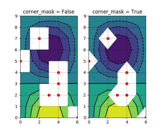
- corner_mask: [ True | False | ‘legacy’ ]
Enable/disable corner masking, which only has an effect if Z is a masked array. If False, any quad touching a masked point is masked out. If True, only the triangular corners of quads nearest those points are always masked out, other triangular corners comprising three unmasked points are contoured as usual. If ‘legacy’, the old contouring algorithm is used, which is equivalent to False and is deprecated, only remaining whilst the new algorithm is tested fully.
If not specified, the default is taken from rcParams[‘contour.corner_mask’], which is True unless it has been modified.
- colors: [ None | string | (mpl_colors) ]
If None, the colormap specified by cmap will be used.
If a string, like ‘r’ or ‘red’, all levels will be plotted in this color.
If a tuple of matplotlib color args (string, float, rgb, etc), different levels will be plotted in different colors in the order specified.
- alpha: float
- The alpha blending value
- cmap: [ None | Colormap ]
- A cm
Colormapinstance or None. If cmap is None and colors is None, a default Colormap is used. - norm: [ None | Normalize ]
- A
matplotlib.colors.Normalizeinstance for scaling data values to colors. If norm is None and colors is None, the default linear scaling is used. - vmin, vmax: [ None | scalar ]
- If not None, either or both of these values will be
supplied to the
matplotlib.colors.Normalizeinstance, overriding the default color scaling based on levels. - levels: [level0, level1, ..., leveln]
- A list of floating point numbers indicating the level
curves to draw, in increasing order; e.g., to draw just
the zero contour pass
levels=[0] - origin: [ None | ‘upper’ | ‘lower’ | ‘image’ ]
If None, the first value of Z will correspond to the lower left corner, location (0,0). If ‘image’, the rc value for
image.originwill be used.This keyword is not active if X and Y are specified in the call to contour.
extent: [ None | (x0,x1,y0,y1) ]
If origin is not None, then extent is interpreted as in
matplotlib.pyplot.imshow(): it gives the outer pixel boundaries. In this case, the position of Z[0,0] is the center of the pixel, not a corner. If origin is None, then (x0, y0) is the position of Z[0,0], and (x1, y1) is the position of Z[-1,-1].This keyword is not active if X and Y are specified in the call to contour.
- locator: [ None | ticker.Locator subclass ]
- If locator is None, the default
MaxNLocatoris used. The locator is used to determine the contour levels if they are not given explicitly via the V argument. - extend: [ ‘neither’ | ‘both’ | ‘min’ | ‘max’ ]
- Unless this is ‘neither’, contour levels are automatically
added to one or both ends of the range so that all data
are included. These added ranges are then mapped to the
special colormap values which default to the ends of the
colormap range, but can be set via
matplotlib.colors.Colormap.set_under()andmatplotlib.colors.Colormap.set_over()methods. - xunits, yunits: [ None | registered units ]
- Override axis units by specifying an instance of a
matplotlib.units.ConversionInterface. - antialiased: [ True | False ]
- enable antialiasing, overriding the defaults. For filled contours, the default is True. For line contours, it is taken from rcParams[‘lines.antialiased’].
- nchunk: [ 0 | integer ]
- If 0, no subdivision of the domain. Specify a positive integer to divide the domain into subdomains of nchunk by nchunk quads. Chunking reduces the maximum length of polygons generated by the contouring algorithm which reduces the rendering workload passed on to the backend and also requires slightly less RAM. It can however introduce rendering artifacts at chunk boundaries depending on the backend, the antialiased flag and value of alpha.
contour-only keyword arguments:
- linewidths: [ None | number | tuple of numbers ]
If linewidths is None, the default width in
lines.linewidthinmatplotlibrcis used.If a number, all levels will be plotted with this linewidth.
If a tuple, different levels will be plotted with different linewidths in the order specified.
- linestyles: [ None | ‘solid’ | ‘dashed’ | ‘dashdot’ | ‘dotted’ ]
If linestyles is None, the default is ‘solid’ unless the lines are monochrome. In that case, negative contours will take their linestyle from the
matplotlibrccontour.negative_linestylesetting.linestyles can also be an iterable of the above strings specifying a set of linestyles to be used. If this iterable is shorter than the number of contour levels it will be repeated as necessary.
contourf-only keyword arguments:
- hatches:
- A list of cross hatch patterns to use on the filled areas. If None, no hatching will be added to the contour. Hatching is supported in the PostScript, PDF, SVG and Agg backends only.
Note: contourf fills intervals that are closed at the top; that is, for boundaries z1 and z2, the filled region is:
z1 < z <= z2
There is one exception: if the lowest boundary coincides with the minimum value of the z array, then that minimum value will be included in the lowest interval.
Examples:
(Source code, png, pdf)
-
matplotlib.pyplot.contourf(*args, **kwargs)¶ Plot contours.
contour()andcontourf()draw contour lines and filled contours, respectively. Except as noted, function signatures and return values are the same for both versions.contourf()differs from the MATLAB version in that it does not draw the polygon edges. To draw edges, add line contours with calls tocontour().Call signatures:
contour(Z)
make a contour plot of an array Z. The level values are chosen automatically.
contour(X,Y,Z)
X, Y specify the (x, y) coordinates of the surface
contour(Z,N)
contour(X,Y,Z,N)
contour up to N automatically-chosen levels.
contour(Z,V)
contour(X,Y,Z,V)
draw contour lines at the values specified in sequence V, which must be in increasing order.
contourf(..., V)
fill the
len(V)-1regions between the values in V, which must be in increasing order.contour(Z, **kwargs)
Use keyword args to control colors, linewidth, origin, cmap ... see below for more details.
X and Y must both be 2-D with the same shape as Z, or they must both be 1-D such that
len(X)is the number of columns in Z andlen(Y)is the number of rows in Z.C = contour(...)returns aQuadContourSetobject.Optional keyword arguments:
- corner_mask: [ True | False | ‘legacy’ ]
Enable/disable corner masking, which only has an effect if Z is a masked array. If False, any quad touching a masked point is masked out. If True, only the triangular corners of quads nearest those points are always masked out, other triangular corners comprising three unmasked points are contoured as usual. If ‘legacy’, the old contouring algorithm is used, which is equivalent to False and is deprecated, only remaining whilst the new algorithm is tested fully.
If not specified, the default is taken from rcParams[‘contour.corner_mask’], which is True unless it has been modified.
- colors: [ None | string | (mpl_colors) ]
If None, the colormap specified by cmap will be used.
If a string, like ‘r’ or ‘red’, all levels will be plotted in this color.
If a tuple of matplotlib color args (string, float, rgb, etc), different levels will be plotted in different colors in the order specified.
- alpha: float
- The alpha blending value
- cmap: [ None | Colormap ]
- A cm
Colormapinstance or None. If cmap is None and colors is None, a default Colormap is used. - norm: [ None | Normalize ]
- A
matplotlib.colors.Normalizeinstance for scaling data values to colors. If norm is None and colors is None, the default linear scaling is used. - vmin, vmax: [ None | scalar ]
- If not None, either or both of these values will be
supplied to the
matplotlib.colors.Normalizeinstance, overriding the default color scaling based on levels. - levels: [level0, level1, ..., leveln]
- A list of floating point numbers indicating the level
curves to draw, in increasing order; e.g., to draw just
the zero contour pass
levels=[0] - origin: [ None | ‘upper’ | ‘lower’ | ‘image’ ]
If None, the first value of Z will correspond to the lower left corner, location (0,0). If ‘image’, the rc value for
image.originwill be used.This keyword is not active if X and Y are specified in the call to contour.
extent: [ None | (x0,x1,y0,y1) ]
If origin is not None, then extent is interpreted as in
matplotlib.pyplot.imshow(): it gives the outer pixel boundaries. In this case, the position of Z[0,0] is the center of the pixel, not a corner. If origin is None, then (x0, y0) is the position of Z[0,0], and (x1, y1) is the position of Z[-1,-1].This keyword is not active if X and Y are specified in the call to contour.
- locator: [ None | ticker.Locator subclass ]
- If locator is None, the default
MaxNLocatoris used. The locator is used to determine the contour levels if they are not given explicitly via the V argument. - extend: [ ‘neither’ | ‘both’ | ‘min’ | ‘max’ ]
- Unless this is ‘neither’, contour levels are automatically
added to one or both ends of the range so that all data
are included. These added ranges are then mapped to the
special colormap values which default to the ends of the
colormap range, but can be set via
matplotlib.colors.Colormap.set_under()andmatplotlib.colors.Colormap.set_over()methods. - xunits, yunits: [ None | registered units ]
- Override axis units by specifying an instance of a
matplotlib.units.ConversionInterface. - antialiased: [ True | False ]
- enable antialiasing, overriding the defaults. For filled contours, the default is True. For line contours, it is taken from rcParams[‘lines.antialiased’].
- nchunk: [ 0 | integer ]
- If 0, no subdivision of the domain. Specify a positive integer to divide the domain into subdomains of nchunk by nchunk quads. Chunking reduces the maximum length of polygons generated by the contouring algorithm which reduces the rendering workload passed on to the backend and also requires slightly less RAM. It can however introduce rendering artifacts at chunk boundaries depending on the backend, the antialiased flag and value of alpha.
contour-only keyword arguments:
- linewidths: [ None | number | tuple of numbers ]
If linewidths is None, the default width in
lines.linewidthinmatplotlibrcis used.If a number, all levels will be plotted with this linewidth.
If a tuple, different levels will be plotted with different linewidths in the order specified.
- linestyles: [ None | ‘solid’ | ‘dashed’ | ‘dashdot’ | ‘dotted’ ]
If linestyles is None, the default is ‘solid’ unless the lines are monochrome. In that case, negative contours will take their linestyle from the
matplotlibrccontour.negative_linestylesetting.linestyles can also be an iterable of the above strings specifying a set of linestyles to be used. If this iterable is shorter than the number of contour levels it will be repeated as necessary.
contourf-only keyword arguments:
- hatches:
- A list of cross hatch patterns to use on the filled areas. If None, no hatching will be added to the contour. Hatching is supported in the PostScript, PDF, SVG and Agg backends only.
Note: contourf fills intervals that are closed at the top; that is, for boundaries z1 and z2, the filled region is:
z1 < z <= z2
There is one exception: if the lowest boundary coincides with the minimum value of the z array, then that minimum value will be included in the lowest interval.
Examples:
(Source code, png, pdf)
-
matplotlib.pyplot.cool()¶ set the default colormap to cool and apply to current image if any. See help(colormaps) for more information
-
matplotlib.pyplot.copper()¶ set the default colormap to copper and apply to current image if any. See help(colormaps) for more information
-
matplotlib.pyplot.csd(x, y, NFFT=None, Fs=None, Fc=None, detrend=None, window=None, noverlap=None, pad_to=None, sides=None, scale_by_freq=None, return_line=None, hold=None, data=None, **kwargs)¶ Plot the cross-spectral density.
Call signature:
csd(x, y, NFFT=256, Fs=2, Fc=0, detrend=mlab.detrend_none,
    window=mlab.window_hanning, noverlap=0, pad_to=None,
    sides='default', scale_by_freq=None, return_line=None, **kwargs)
The cross spectral density
 by Welch’s average
periodogram method. The vectors x and y are divided into
NFFT length segments. Each segment is detrended by function
detrend and windowed by function window. noverlap gives
the length of the overlap between segments. The product of
the direct FFTs of x and y are averaged over each segment
to compute , with a scaling to correct for power
loss due to windowing.
by Welch’s average
periodogram method. The vectors x and y are divided into
NFFT length segments. Each segment is detrended by function
detrend and windowed by function window. noverlap gives
the length of the overlap between segments. The product of
the direct FFTs of x and y are averaged over each segment
to compute , with a scaling to correct for power
loss due to windowing.If len(x) < NFFT or len(y) < NFFT, they will be zero padded to NFFT.
Parameters: x, y : 1-D arrays or sequences
Arrays or sequences containing the data
Fs : scalar
The sampling frequency (samples per time unit). It is used to calculate the Fourier frequencies, freqs, in cycles per time unit. The default value is 2.
window : callable or ndarray
A function or a vector of length NFFT. To create window vectors see
window_hanning(),window_none(),numpy.blackman(),numpy.hamming(),numpy.bartlett(),scipy.signal(),scipy.signal.get_window(), etc. The default iswindow_hanning(). If a function is passed as the argument, it must take a data segment as an argument and return the windowed version of the segment.sides : [ ‘default’ | ‘onesided’ | ‘twosided’ ]
Specifies which sides of the spectrum to return. Default gives the default behavior, which returns one-sided for real data and both for complex data. ‘onesided’ forces the return of a one-sided spectrum, while ‘twosided’ forces two-sided.
pad_to : integer
The number of points to which the data segment is padded when performing the FFT. This can be different from NFFT, which specifies the number of data points used. While not increasing the actual resolution of the spectrum (the minimum distance between resolvable peaks), this can give more points in the plot, allowing for more detail. This corresponds to the n parameter in the call to fft(). The default is None, which sets pad_to equal to NFFT
NFFT : integer
The number of data points used in each block for the FFT. A power 2 is most efficient. The default value is 256. This should NOT be used to get zero padding, or the scaling of the result will be incorrect. Use pad_to for this instead.
detrend : {‘default’, ‘constant’, ‘mean’, ‘linear’, ‘none’} or callable
The function applied to each segment before fft-ing, designed to remove the mean or linear trend. Unlike in MATLAB, where the detrend parameter is a vector, in matplotlib is it a function. The
pylabmodule definesdetrend_none(),detrend_mean(), anddetrend_linear(), but you can use a custom function as well. You can also use a string to choose one of the functions. ‘default’, ‘constant’, and ‘mean’ calldetrend_mean(). ‘linear’ callsdetrend_linear(). ‘none’ callsdetrend_none().scale_by_freq : boolean, optional
Specifies whether the resulting density values should be scaled by the scaling frequency, which gives density in units of Hz^-1. This allows for integration over the returned frequency values. The default is True for MATLAB compatibility.
noverlap : integer
The number of points of overlap between segments. The default value is 0 (no overlap).
Fc : integer
The center frequency of x (defaults to 0), which offsets the x extents of the plot to reflect the frequency range used when a signal is acquired and then filtered and downsampled to baseband.
return_line : bool
Whether to include the line object plotted in the returned values. Default is False.
**kwargs :
Keyword arguments control the
Line2Dproperties:Property Description agg_filterunknown alphafloat (0.0 transparent through 1.0 opaque) animated[True | False] antialiasedor aa[True | False] axesan Axesinstanceclip_boxa matplotlib.transforms.Bboxinstanceclip_on[True | False] clip_path[ ( Path,Transform) |Patch| None ]coloror cany matplotlib color containsa callable function dash_capstyle[‘butt’ | ‘round’ | ‘projecting’] dash_joinstyle[‘miter’ | ‘round’ | ‘bevel’] dashessequence of on/off ink in points drawstyle[‘default’ | ‘steps’ | ‘steps-pre’ | ‘steps-mid’ | ‘steps-post’] figurea matplotlib.figure.Figureinstancefillstyle[‘full’ | ‘left’ | ‘right’ | ‘bottom’ | ‘top’ | ‘none’] gidan id string labelstring or anything printable with ‘%s’ conversion. linestyleor ls[‘solid’ | ‘dashed’, ‘dashdot’, ‘dotted’ | (offset, on-off-dash-seq) | '-'|'--'|'-.'|':'|'None'|' '|'']linewidthor lwfloat value in points markerA valid marker stylemarkeredgecoloror mecany matplotlib color markeredgewidthor mewfloat value in points markerfacecoloror mfcany matplotlib color markerfacecoloraltor mfcaltany matplotlib color markersizeor msfloat markevery[None | int | length-2 tuple of int | slice | list/array of int | float | length-2 tuple of float] path_effectsunknown pickerfloat distance in points or callable pick function fn(artist, event)pickradiusfloat distance in points rasterized[True | False | None] sketch_paramsunknown snapunknown solid_capstyle[‘butt’ | ‘round’ | ‘projecting’] solid_joinstyle[‘miter’ | ‘round’ | ‘bevel’] transforma matplotlib.transforms.Transforminstanceurla url string visible[True | False] xdata1D array ydata1D array zorderany number Returns: Pxy : 1-D array
The values for the cross spectrum
P_{xy}before scaling (complex valued)freqs : 1-D array
The frequencies corresponding to the elements in Pxy
line : a
Line2DinstanceThe line created by this function. Only returned if return_line is True.
See also
Notes
For plotting, the power is plotted as
 for decibels, though
 P_{xy}itself is returned.References
Bendat & Piersol – Random Data: Analysis and Measurement Procedures, John Wiley & Sons (1986)
Examples
(Source code, png, pdf)
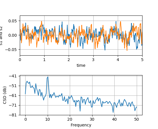
-
matplotlib.pyplot.delaxes(*args)¶ Remove an axes from the current figure. If ax doesn’t exist, an error will be raised.
delaxes(): delete the current axes
-
matplotlib.pyplot.disconnect(cid)¶ Disconnect callback id cid
Example usage:
cid = canvas.mpl_connect('button_press_event', on_press)
#...later
canvas.mpl_disconnect(cid)
-
matplotlib.pyplot.draw()¶ Redraw the current figure.
This is used to update a figure that has been altered, but not automatically re-drawn. If interactive mode is on (
ion()), this should be only rarely needed, but there may be ways to modify the state of a figure without marking it asstale. Please report these cases as bugs.A more object-oriented alternative, given any
Figureinstance,fig, that was created using apyplotfunction, is:fig.canvas.draw_idle()
-
matplotlib.pyplot.errorbar(x, y, yerr=None, xerr=None, fmt='', ecolor=None, elinewidth=None, capsize=None, barsabove=False, lolims=False, uplims=False, xlolims=False, xuplims=False, errorevery=1, capthick=None, hold=None, data=None, **kwargs)¶ Plot an errorbar graph.
Plot x versus y with error deltas in yerr and xerr. Vertical errorbars are plotted if yerr is not None. Horizontal errorbars are plotted if xerr is not None.
x, y, xerr, and yerr can all be scalars, which plots a single error bar at x, y.
Parameters: x : scalar or array-like
y : scalar or array-like
xerr/yerr : scalar or array-like, shape(N,) or shape(2,N), optional
If a scalar number, len(N) array-like object, or a N-element array-like object, errorbars are drawn at +/-value relative to the data. Default is None.
If a sequence of shape 2xN, errorbars are drawn at -row1 and +row2 relative to the data.
fmt : plot format string, optional, default: None
The plot format symbol. If fmt is ‘none’ (case-insensitive), only the errorbars are plotted. This is used for adding errorbars to a bar plot, for example. Default is ‘’, an empty plot format string; properties are then identical to the defaults for
plot().ecolor : mpl color, optional, default: None
A matplotlib color arg which gives the color the errorbar lines; if None, use the color of the line connecting the markers.
elinewidth : scalar, optional, default: None
The linewidth of the errorbar lines. If None, use the linewidth.
capsize : scalar, optional, default: None
The length of the error bar caps in points; if None, it will take the value from
errorbar.capsizercParam.capthick : scalar, optional, default: None
An alias kwarg to markeredgewidth (a.k.a. - mew). This setting is a more sensible name for the property that controls the thickness of the error bar cap in points. For backwards compatibility, if mew or markeredgewidth are given, then they will over-ride capthick. This may change in future releases.
barsabove : bool, optional, default: False
if True , will plot the errorbars above the plot symbols. Default is below.
lolims / uplims / xlolims / xuplims : bool, optional, default:None
These arguments can be used to indicate that a value gives only upper/lower limits. In that case a caret symbol is used to indicate this. lims-arguments may be of the same type as xerr and yerr. To use limits with inverted axes,
set_xlim()orset_ylim()must be called beforeerrorbar().errorevery : positive integer, optional, default:1
subsamples the errorbars. e.g., if errorevery=5, errorbars for every 5-th datapoint will be plotted. The data plot itself still shows all data points.
Returns: plotline :
Line2Dinstancex, y plot markers and/or line
caplines : list of
Line2Dinstanceserror bar cap
barlinecols : list of
LineCollectionhorizontal and vertical error ranges.
Other Parameters: kwargs : All other keyword arguments are passed on to the plot
command for the markers. For example, this code makes big red squares with thick green edges:
x,y,yerr = rand(3,10)
errorbar(x, y, yerr, marker='s', mfc='red',
         mec='green', ms=20, mew=4)
where mfc, mec, ms and mew are aliases for the longer property names, markerfacecolor, markeredgecolor, markersize and markeredgewidth.
valid kwargs for the marker properties are
Property Description agg_filterunknown alphafloat (0.0 transparent through 1.0 opaque) animated[True | False] antialiasedor aa[True | False] axesan Axesinstanceclip_boxa matplotlib.transforms.Bboxinstanceclip_on[True | False] clip_path[ ( Path,Transform) |Patch| None ]coloror cany matplotlib color containsa callable function dash_capstyle[‘butt’ | ‘round’ | ‘projecting’] dash_joinstyle[‘miter’ | ‘round’ | ‘bevel’] dashessequence of on/off ink in points drawstyle[‘default’ | ‘steps’ | ‘steps-pre’ | ‘steps-mid’ | ‘steps-post’] figurea matplotlib.figure.Figureinstancefillstyle[‘full’ | ‘left’ | ‘right’ | ‘bottom’ | ‘top’ | ‘none’] gidan id string labelstring or anything printable with ‘%s’ conversion. linestyleor ls[‘solid’ | ‘dashed’, ‘dashdot’, ‘dotted’ | (offset, on-off-dash-seq) | '-'|'--'|'-.'|':'|'None'|' '|'']linewidthor lwfloat value in points markerA valid marker stylemarkeredgecoloror mecany matplotlib color markeredgewidthor mewfloat value in points markerfacecoloror mfcany matplotlib color markerfacecoloraltor mfcaltany matplotlib color markersizeor msfloat markevery[None | int | length-2 tuple of int | slice | list/array of int | float | length-2 tuple of float] path_effectsunknown pickerfloat distance in points or callable pick function fn(artist, event)pickradiusfloat distance in points rasterized[True | False | None] sketch_paramsunknown snapunknown solid_capstyle[‘butt’ | ‘round’ | ‘projecting’] solid_joinstyle[‘miter’ | ‘round’ | ‘bevel’] transforma matplotlib.transforms.Transforminstanceurla url string visible[True | False] xdata1D array ydata1D array zorderany number Examples
(Source code, png, pdf)
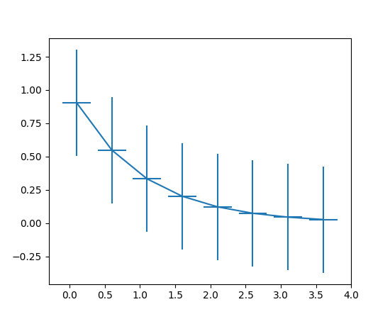
Note
In addition to the above described arguments, this function can take a data keyword argument. If such a data argument is given, the following arguments are replaced by data[<arg>]:
- All arguments with the following names: ‘x’, ‘xerr’, ‘y’, ‘yerr’.
-
matplotlib.pyplot.eventplot(positions, orientation='horizontal', lineoffsets=1, linelengths=1, linewidths=None, colors=None, linestyles='solid', hold=None, data=None, **kwargs)¶ Plot identical parallel lines at specific positions.
Plot parallel lines at the given positions. positions should be a 1D or 2D array-like object, with each row corresponding to a row or column of lines.
This type of plot is commonly used in neuroscience for representing neural events, where it is commonly called a spike raster, dot raster, or raster plot.
However, it is useful in any situation where you wish to show the timing or position of multiple sets of discrete events, such as the arrival times of people to a business on each day of the month or the date of hurricanes each year of the last century.
- orientation : [ ‘horizontal’ | ‘vertical’ ]
- ‘horizontal’ : the lines will be vertical and arranged in rows ‘vertical’ : lines will be horizontal and arranged in columns
- lineoffsets :
- A float or array-like containing floats.
- linelengths :
- A float or array-like containing floats.
- linewidths :
- A float or array-like containing floats.
- colors
- must be a sequence of RGBA tuples (e.g., arbitrary color strings, etc, not allowed) or a list of such sequences
- linestyles :
- [ ‘solid’ | ‘dashed’ | ‘dashdot’ | ‘dotted’ ] or an array of these values
For linelengths, linewidths, colors, and linestyles, if only a single value is given, that value is applied to all lines. If an array-like is given, it must have the same length as positions, and each value will be applied to the corresponding row or column in positions.
Returns a list of
matplotlib.collections.EventCollectionobjects that were added.kwargs are
LineCollectionproperties:Property Description agg_filterunknown alphafloat or None animated[True | False] antialiasedor antialiasedsBoolean or sequence of booleans arrayunknown axesan Axesinstanceclima length 2 sequence of floats clip_boxa matplotlib.transforms.Bboxinstanceclip_on[True | False] clip_path[ ( Path,Transform) |Patch| None ]cmapa colormap or registered colormap name colormatplotlib color arg or sequence of rgba tuples containsa callable function edgecoloror edgecolorsmatplotlib color spec or sequence of specs facecoloror facecolorsmatplotlib color spec or sequence of specs figurea matplotlib.figure.Figureinstancegidan id string hatch[ ‘/’ | ‘\’ | ‘|’ | ‘-‘ | ‘+’ | ‘x’ | ‘o’ | ‘O’ | ‘.’ | ‘*’ ] labelstring or anything printable with ‘%s’ conversion. linestyleor dashes or linestyles[‘solid’ | ‘dashed’, ‘dashdot’, ‘dotted’ | (offset, on-off-dash-seq) | '-'|'--'|'-.'|':'|'None'|' '|'']linewidthor linewidths or lwfloat or sequence of floats normunknown offset_positionunknown offsetsfloat or sequence of floats path_effectsunknown pathsunknown picker[None|float|boolean|callable] pickradiusunknown rasterized[True | False | None] segmentsunknown sketch_paramsunknown snapunknown transformTransforminstanceurla url string urlsunknown vertsunknown visible[True | False] zorderany number Example:
(Source code, png, pdf)
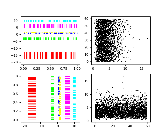
Note
In addition to the above described arguments, this function can take a data keyword argument. If such a data argument is given, the following arguments are replaced by data[<arg>]:
- All arguments with the following names: ‘colors’, ‘linelengths’, ‘lineoffsets’, ‘linestyles’, ‘linewidths’, ‘positions’.
-
matplotlib.pyplot.figimage(*args, **kwargs)¶ Adds a non-resampled image to the figure.
call signatures:
figimage(X, **kwargs)
adds a non-resampled array X to the figure.
figimage(X, xo, yo)
with pixel offsets xo, yo,
X must be a float array:
- If X is MxN, assume luminance (grayscale)
- If X is MxNx3, assume RGB
- If X is MxNx4, assume RGBA
Optional keyword arguments:
Keyword Description resize a boolean, True or False. If “True”, then re-size the Figure to match the given image size. xo or yo An integer, the x and y image offset in pixels cmap a matplotlib.colors.Colormapinstance, e.g., cm.jet. If None, default to the rcimage.cmapvaluenorm a matplotlib.colors.Normalizeinstance. The default is normalization(). This scales luminance -> 0-1vmin|vmax are used to scale a luminance image to 0-1. If either is None, the min and max of the luminance values will be used. Note if you pass a norm instance, the settings for vmin and vmax will be ignored. alpha the alpha blending value, default is None origin [ ‘upper’ | ‘lower’ ] Indicates where the [0,0] index of the array is in the upper left or lower left corner of the axes. Defaults to the rc image.origin value figimage complements the axes image (
imshow()) which will be resampled to fit the current axes. If you want a resampled image to fill the entire figure, you can define anAxeswith extent [0,0,1,1].An
matplotlib.image.FigureImageinstance is returned.(Source code, png, pdf)

Additional kwargs are Artist kwargs passed on to
FigureImage
-
matplotlib.pyplot.figlegend(handles, labels, loc, **kwargs)¶ Place a legend in the figure.
- labels
- a sequence of strings
- handles
- a sequence of
Line2DorPatchinstances - loc
- can be a string or an integer specifying the legend location
A
matplotlib.legend.Legendinstance is returned.Example:
figlegend( (line1, line2, line3),
           ('label1', 'label2', 'label3'),
           'upper right' )
-
matplotlib.pyplot.fignum_exists(num)
-
matplotlib.pyplot.figtext(*args, **kwargs)¶ Add text to figure.
Call signature:
text(x, y, s, fontdict=None, **kwargs)
Add text to figure at location x, y (relative 0-1 coords). See
text()for the meaning of the other arguments.kwargs control the
Textproperties:Property Description agg_filterunknown alphafloat (0.0 transparent through 1.0 opaque) animated[True | False] axesan Axesinstancebackgroundcolorany matplotlib color bboxFancyBboxPatch prop dict clip_boxa matplotlib.transforms.Bboxinstanceclip_on[True | False] clip_path[ ( Path,Transform) |Patch| None ]colorany matplotlib color containsa callable function familyor fontfamily or fontname or name[FONTNAME | ‘serif’ | ‘sans-serif’ | ‘cursive’ | ‘fantasy’ | ‘monospace’ ] figurea matplotlib.figure.Figureinstancefontpropertiesor font_propertiesa matplotlib.font_manager.FontPropertiesinstancegidan id string horizontalalignmentor ha[ ‘center’ | ‘right’ | ‘left’ ] labelstring or anything printable with ‘%s’ conversion. linespacingfloat (multiple of font size) multialignment[‘left’ | ‘right’ | ‘center’ ] path_effectsunknown picker[None|float|boolean|callable] position(x,y) rasterized[True | False | None] rotation[ angle in degrees | ‘vertical’ | ‘horizontal’ ] rotation_modeunknown sizeor fontsize[size in points | ‘xx-small’ | ‘x-small’ | ‘small’ | ‘medium’ | ‘large’ | ‘x-large’ | ‘xx-large’ ] sketch_paramsunknown snapunknown stretchor fontstretch[a numeric value in range 0-1000 | ‘ultra-condensed’ | ‘extra-condensed’ | ‘condensed’ | ‘semi-condensed’ | ‘normal’ | ‘semi-expanded’ | ‘expanded’ | ‘extra-expanded’ | ‘ultra-expanded’ ] styleor fontstyle[ ‘normal’ | ‘italic’ | ‘oblique’] textstring or anything printable with ‘%s’ conversion. transformTransforminstanceurla url string usetexunknown variantor fontvariant[ ‘normal’ | ‘small-caps’ ] verticalalignmentor ma or va[ ‘center’ | ‘top’ | ‘bottom’ | ‘baseline’ ] visible[True | False] weightor fontweight[a numeric value in range 0-1000 | ‘ultralight’ | ‘light’ | ‘normal’ | ‘regular’ | ‘book’ | ‘medium’ | ‘roman’ | ‘semibold’ | ‘demibold’ | ‘demi’ | ‘bold’ | ‘heavy’ | ‘extra bold’ | ‘black’ ] wrapunknown xfloat yfloat zorderany number
-
matplotlib.pyplot.figure(num=None, figsize=None, dpi=None, facecolor=None, edgecolor=None, frameon=True, FigureClass=<class 'matplotlib.figure.Figure'>, **kwargs)¶ Creates a new figure.
Parameters: num : integer or string, optional, default: none
If not provided, a new figure will be created, and the figure number will be incremented. The figure objects holds this number in a
numberattribute. If num is provided, and a figure with this id already exists, make it active, and returns a reference to it. If this figure does not exists, create it and returns it. If num is a string, the window title will be set to this figure’snum.figsize : tuple of integers, optional, default: None
width, height in inches. If not provided, defaults to rc figure.figsize.
dpi : integer, optional, default: None
resolution of the figure. If not provided, defaults to rc figure.dpi.
facecolor :
the background color. If not provided, defaults to rc figure.facecolor
edgecolor :
the border color. If not provided, defaults to rc figure.edgecolor
Returns: figure : Figure
The Figure instance returned will also be passed to new_figure_manager in the backends, which allows to hook custom Figure classes into the pylab interface. Additional kwargs will be passed to the figure init function.
Notes
If you are creating many figures, make sure you explicitly call “close” on the figures you are not using, because this will enable pylab to properly clean up the memory.
rcParams defines the default values, which can be modified in the matplotlibrc file
-
matplotlib.pyplot.fill(*args, **kwargs)¶ Plot filled polygons.
Parameters: args : a variable length argument
It allowing for multiple x, y pairs with an optional color format string; see
plot()for details on the argument parsing. For example, each of the following is legal:ax.fill(x, y) ax.fill(x, y, "b") ax.fill(x, y, "b", x, y, "r")
An arbitrary number of x, y, color groups can be specified:: ax.fill(x1, y1, ‘g’, x2, y2, ‘r’)
Returns: a list of
PatchOther Parameters: kwargs :
PolygonpropertiesNotes
The same color strings that
plot()supports are supported by the fill format string.If you would like to fill below a curve, e.g., shade a region between 0 and y along x, use
fill_between()Examples
(Source code, png, pdf)
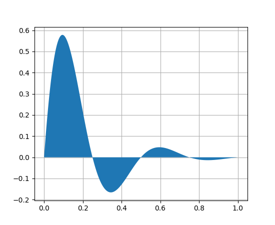
Note
In addition to the above described arguments, this function can take a data keyword argument. If such a data argument is given, the following arguments are replaced by data[<arg>]:
- All arguments with the following names: ‘x’, ‘y’.
-
matplotlib.pyplot.fill_between(x, y1, y2=0, where=None, interpolate=False, step=None, hold=None, data=None, **kwargs)¶ Make filled polygons between two curves.
Create a
PolyCollectionfilling the regions between y1 and y2 wherewhere==TrueParameters: x : array
An N-length array of the x data
y1 : array
An N-length array (or scalar) of the y data
y2 : array
An N-length array (or scalar) of the y data
where : array, optional
If
None, default to fill between everywhere. If notNone, it is an N-length numpy boolean array and the fill will only happen over the regions wherewhere==True.interpolate : bool, optional
If
True, interpolate between the two lines to find the precise point of intersection. Otherwise, the start and end points of the filled region will only occur on explicit values in the x array.step : {‘pre’, ‘post’, ‘mid’}, optional
If not None, fill with step logic.
See also
- In addition to the above described arguments, this function can take a data keyword argument. If such a data argument is given, the following arguments are replaced by data[<arg>]: * All arguments with the following names: ‘where’, ‘x’, ‘y1’, ‘y2’.
Notes
Additional Keyword args passed on to the
PolyCollection.kwargs control the
Polygonproperties:Property Description agg_filterunknown alphafloat or None animated[True | False] antialiasedor antialiasedsBoolean or sequence of booleans arrayunknown axesan Axesinstanceclima length 2 sequence of floats clip_boxa matplotlib.transforms.Bboxinstanceclip_on[True | False] clip_path[ ( Path,Transform) |Patch| None ]cmapa colormap or registered colormap name colormatplotlib color arg or sequence of rgba tuples containsa callable function edgecoloror edgecolorsmatplotlib color spec or sequence of specs facecoloror facecolorsmatplotlib color spec or sequence of specs figurea matplotlib.figure.Figureinstancegidan id string hatch[ ‘/’ | ‘\’ | ‘|’ | ‘-‘ | ‘+’ | ‘x’ | ‘o’ | ‘O’ | ‘.’ | ‘*’ ] labelstring or anything printable with ‘%s’ conversion. linestyleor dashes or linestyles[‘solid’ | ‘dashed’, ‘dashdot’, ‘dotted’ | (offset, on-off-dash-seq) | '-'|'--'|'-.'|':'|'None'|' '|'']linewidthor linewidths or lwfloat or sequence of floats normunknown offset_positionunknown offsetsfloat or sequence of floats path_effectsunknown picker[None|float|boolean|callable] pickradiusunknown rasterized[True | False | None] sketch_paramsunknown snapunknown transformTransforminstanceurla url string urlsunknown visible[True | False] zorderany number Examples
-
matplotlib.pyplot.fill_betweenx(y, x1, x2=0, where=None, step=None, hold=None, data=None, **kwargs)¶ Make filled polygons between two horizontal curves.
Create a
PolyCollectionfilling the regions between x1 and x2 wherewhere==TrueParameters: y : array
An N-length array of the y data
x1 : array
An N-length array (or scalar) of the x data
x2 : array, optional
An N-length array (or scalar) of the x data
where : array, optional
If None, default to fill between everywhere. If not None, it is a N length numpy boolean array and the fill will only happen over the regions where
where==Truestep : {‘pre’, ‘post’, ‘mid’}, optional
If not None, fill with step logic.
See also
- In addition to the above described arguments, this function can take a data keyword argument. If such a data argument is given, the following arguments are replaced by data[<arg>]: * All arguments with the following names: ‘where’, ‘x1’, ‘x2’, ‘y’.
Notes
- keyword args passed on to the
PolyCollection
kwargs control the
Polygonproperties:Property Description agg_filterunknown alphafloat or None animated[True | False] antialiasedor antialiasedsBoolean or sequence of booleans arrayunknown axesan Axesinstanceclima length 2 sequence of floats clip_boxa matplotlib.transforms.Bboxinstanceclip_on[True | False] clip_path[ ( Path,Transform) |Patch| None ]cmapa colormap or registered colormap name colormatplotlib color arg or sequence of rgba tuples containsa callable function edgecoloror edgecolorsmatplotlib color spec or sequence of specs facecoloror facecolorsmatplotlib color spec or sequence of specs figurea matplotlib.figure.Figureinstancegidan id string hatch[ ‘/’ | ‘\’ | ‘|’ | ‘-‘ | ‘+’ | ‘x’ | ‘o’ | ‘O’ | ‘.’ | ‘*’ ] labelstring or anything printable with ‘%s’ conversion. linestyleor dashes or linestyles[‘solid’ | ‘dashed’, ‘dashdot’, ‘dotted’ | (offset, on-off-dash-seq) | '-'|'--'|'-.'|':'|'None'|' '|'']linewidthor linewidths or lwfloat or sequence of floats normunknown offset_positionunknown offsetsfloat or sequence of floats path_effectsunknown picker[None|float|boolean|callable] pickradiusunknown rasterized[True | False | None] sketch_paramsunknown snapunknown transformTransforminstanceurla url string urlsunknown visible[True | False] zorderany number Examples
-
matplotlib.pyplot.findobj(o=None, match=None, include_self=True)¶ Find artist objects.
Recursively find all
Artistinstances contained in self.match can be
- None: return all objects contained in artist.
- function with signature
boolean = match(artist)used to filter matches - class instance: e.g., Line2D. Only return artists of class type.
If include_self is True (default), include self in the list to be checked for a match.
-
matplotlib.pyplot.flag()¶ set the default colormap to flag and apply to current image if any. See help(colormaps) for more information
-
matplotlib.pyplot.gca(**kwargs)¶ Get the current
Axesinstance on the current figure matching the given keyword args, or create one.Examples
To get the current polar axes on the current figure:
plt.gca(projection='polar')
If the current axes doesn’t exist, or isn’t a polar one, the appropriate axes will be created and then returned.
-
matplotlib.pyplot.gcf()¶ Get a reference to the current figure.
-
matplotlib.pyplot.gci()¶ Get the current colorable artist. Specifically, returns the current
ScalarMappableinstance (image or patch collection), or None if no images or patch collections have been defined. The commandsimshow()andfigimage()createImageinstances, and the commandspcolor()andscatter()createCollectioninstances. The current image is an attribute of the current axes, or the nearest earlier axes in the current figure that contains an image.
-
matplotlib.pyplot.get_current_fig_manager()
-
matplotlib.pyplot.get_figlabels()¶ Return a list of existing figure labels.
-
matplotlib.pyplot.get_fignums()¶ Return a list of existing figure numbers.
-
matplotlib.pyplot.get_plot_commands()¶ Get a sorted list of all of the plotting commands.
-
matplotlib.pyplot.ginput(*args, **kwargs)¶ Blocking call to interact with the figure.
This will wait for n clicks from the user and return a list of the coordinates of each click.
If timeout is zero or negative, does not timeout.
If n is zero or negative, accumulate clicks until a middle click (or potentially both mouse buttons at once) terminates the input.
Right clicking cancels last input.
The buttons used for the various actions (adding points, removing points, terminating the inputs) can be overriden via the arguments mouse_add, mouse_pop and mouse_stop, that give the associated mouse button: 1 for left, 2 for middle, 3 for right.
The keyboard can also be used to select points in case your mouse does not have one or more of the buttons. The delete and backspace keys act like right clicking (i.e., remove last point), the enter key terminates input and any other key (not already used by the window manager) selects a point.
-
matplotlib.pyplot.gray()¶ set the default colormap to gray and apply to current image if any. See help(colormaps) for more information
-
matplotlib.pyplot.grid(b=None, which='major', axis='both', **kwargs)¶ Turn the axes grids on or off.
Set the axes grids on or off; b is a boolean. (For MATLAB compatibility, b may also be a string, ‘on’ or ‘off’.)
If b is None and
len(kwargs)==0, toggle the grid state. If kwargs are supplied, it is assumed that you want a grid and b is thus set to True.which can be ‘major’ (default), ‘minor’, or ‘both’ to control whether major tick grids, minor tick grids, or both are affected.
axis can be ‘both’ (default), ‘x’, or ‘y’ to control which set of gridlines are drawn.
kwargs are used to set the grid line properties, e.g.,:
ax.grid(color='r', linestyle='-', linewidth=2)
Valid
Line2Dkwargs areProperty Description agg_filterunknown alphafloat (0.0 transparent through 1.0 opaque) animated[True | False] antialiasedor aa[True | False] axesan Axesinstanceclip_boxa matplotlib.transforms.Bboxinstanceclip_on[True | False] clip_path[ ( Path,Transform) |Patch| None ]coloror cany matplotlib color containsa callable function dash_capstyle[‘butt’ | ‘round’ | ‘projecting’] dash_joinstyle[‘miter’ | ‘round’ | ‘bevel’] dashessequence of on/off ink in points drawstyle[‘default’ | ‘steps’ | ‘steps-pre’ | ‘steps-mid’ | ‘steps-post’] figurea matplotlib.figure.Figureinstancefillstyle[‘full’ | ‘left’ | ‘right’ | ‘bottom’ | ‘top’ | ‘none’] gidan id string labelstring or anything printable with ‘%s’ conversion. linestyleor ls[‘solid’ | ‘dashed’, ‘dashdot’, ‘dotted’ | (offset, on-off-dash-seq) | '-'|'--'|'-.'|':'|'None'|' '|'']linewidthor lwfloat value in points markerA valid marker stylemarkeredgecoloror mecany matplotlib color markeredgewidthor mewfloat value in points markerfacecoloror mfcany matplotlib color markerfacecoloraltor mfcaltany matplotlib color markersizeor msfloat markevery[None | int | length-2 tuple of int | slice | list/array of int | float | length-2 tuple of float] path_effectsunknown pickerfloat distance in points or callable pick function fn(artist, event)pickradiusfloat distance in points rasterized[True | False | None] sketch_paramsunknown snapunknown solid_capstyle[‘butt’ | ‘round’ | ‘projecting’] solid_joinstyle[‘miter’ | ‘round’ | ‘bevel’] transforma matplotlib.transforms.Transforminstanceurla url string visible[True | False] xdata1D array ydata1D array zorderany number
-
matplotlib.pyplot.hexbin(x, y, C=None, gridsize=100, bins=None, xscale='linear', yscale='linear', extent=None, cmap=None, norm=None, vmin=None, vmax=None, alpha=None, linewidths=None, edgecolors='none', reduce_C_function=<function mean>, mincnt=None, marginals=False, hold=None, data=None, **kwargs)¶ Make a hexagonal binning plot.
Make a hexagonal binning plot of x versus y, where x, y are 1-D sequences of the same length, N. If C is None (the default), this is a histogram of the number of occurences of the observations at (x[i],y[i]).
If C is specified, it specifies values at the coordinate (x[i],y[i]). These values are accumulated for each hexagonal bin and then reduced according to reduce_C_function, which defaults to numpy’s mean function (np.mean). (If C is specified, it must also be a 1-D sequence of the same length as x and y.)
Parameters: x, y : array or masked array
C : array or masked array, optional, default is None
gridsize : int or (int, int), optional, default is 100
The number of hexagons in the x-direction, default is 100. The corresponding number of hexagons in the y-direction is chosen such that the hexagons are approximately regular. Alternatively, gridsize can be a tuple with two elements specifying the number of hexagons in the x-direction and the y-direction.
bins : {‘log’} or int or sequence, optional, default is None
If None, no binning is applied; the color of each hexagon directly corresponds to its count value.
If ‘log’, use a logarithmic scale for the color map. Internally,
 is used to
determine the hexagon color.
is used to
determine the hexagon color.If an integer, divide the counts in the specified number of bins, and color the hexagons accordingly.
If a sequence of values, the values of the lower bound of the bins to be used.
xscale : {‘linear’, ‘log’}, optional, default is ‘linear’
Use a linear or log10 scale on the horizontal axis.
yscale : {‘linear’, ‘log’}, optional, default is ‘linear’
Use a linear or log10 scale on the vertical axis.
mincnt : int > 0, optional, default is None
If not None, only display cells with more than mincnt number of points in the cell
marginals : bool, optional, default is False
if marginals is True, plot the marginal density as colormapped rectagles along the bottom of the x-axis and left of the y-axis
extent : scalar, optional, default is None
The limits of the bins. The default assigns the limits based on gridsize, x, y, xscale and yscale.
If xscale or yscale is set to ‘log’, the limits are expected to be the exponent for a power of 10. E.g. for x-limits of 1 and 50 in ‘linear’ scale and y-limits of 10 and 1000 in ‘log’ scale, enter (1, 50, 1, 3).
Order of scalars is (left, right, bottom, top).
Returns: object
a
PolyCollectioninstance; useget_array()on thisPolyCollectionto get the counts in each hexagon.If marginals is True, horizontal bar and vertical bar (both PolyCollections) will be attached to the return collection as attributes hbar and vbar.
Other Parameters: cmap : object, optional, default is None
a
matplotlib.colors.Colormapinstance. If None, defaults to rcimage.cmap.norm : object, optional, default is None
matplotlib.colors.Normalizeinstance is used to scale luminance data to 0,1.vmin, vmax : scalar, optional, default is None
vmin and vmax are used in conjunction with norm to normalize luminance data. If None, the min and max of the color array C are used. Note if you pass a norm instance your settings for vmin and vmax will be ignored.
alpha : scalar between 0 and 1, optional, default is None
the alpha value for the patches
linewidths : scalar, optional, default is None
If None, defaults to 1.0.
edgecolors : {‘none’} or mpl color, optional, default is ‘none’
If ‘none’, draws the edges in the same color as the fill color. This is the default, as it avoids unsightly unpainted pixels between the hexagons.
If None, draws outlines in the default color.
If a matplotlib color arg, draws outlines in the specified color.
Notes
The standard descriptions of all the
Collectionparameters:Property Description agg_filterunknown alphafloat or None animated[True | False] antialiasedor antialiasedsBoolean or sequence of booleans arrayunknown axesan Axesinstanceclima length 2 sequence of floats clip_boxa matplotlib.transforms.Bboxinstanceclip_on[True | False] clip_path[ ( Path,Transform) |Patch| None ]cmapa colormap or registered colormap name colormatplotlib color arg or sequence of rgba tuples containsa callable function edgecoloror edgecolorsmatplotlib color spec or sequence of specs facecoloror facecolorsmatplotlib color spec or sequence of specs figurea matplotlib.figure.Figureinstancegidan id string hatch[ ‘/’ | ‘\’ | ‘|’ | ‘-‘ | ‘+’ | ‘x’ | ‘o’ | ‘O’ | ‘.’ | ‘*’ ] labelstring or anything printable with ‘%s’ conversion. linestyleor dashes or linestyles[‘solid’ | ‘dashed’, ‘dashdot’, ‘dotted’ | (offset, on-off-dash-seq) | '-'|'--'|'-.'|':'|'None'|' '|'']linewidthor linewidths or lwfloat or sequence of floats normunknown offset_positionunknown offsetsfloat or sequence of floats path_effectsunknown picker[None|float|boolean|callable] pickradiusunknown rasterized[True | False | None] sketch_paramsunknown snapunknown transformTransforminstanceurla url string urlsunknown visible[True | False] zorderany number Note
In addition to the above described arguments, this function can take a data keyword argument. If such a data argument is given, the following arguments are replaced by data[<arg>]:
- All arguments with the following names: ‘x’, ‘y’.
Examples
(Source code, png, pdf)
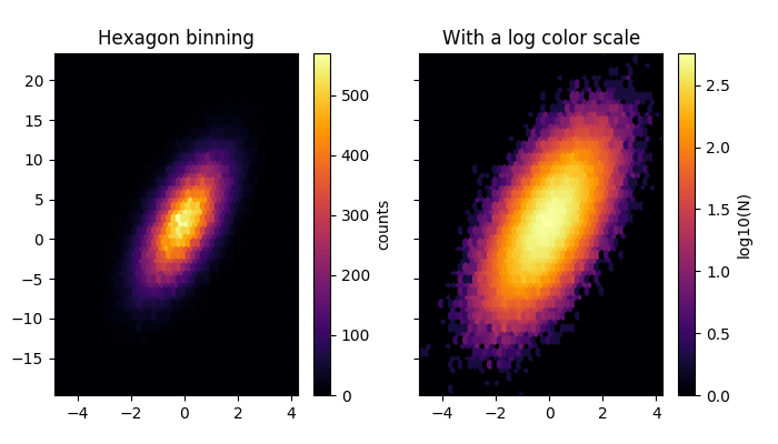
-
matplotlib.pyplot.hist(x, bins=None, range=None, normed=False, weights=None, cumulative=False, bottom=None, histtype='bar', align='mid', orientation='vertical', rwidth=None, log=False, color=None, label=None, stacked=False, hold=None, data=None, **kwargs)¶ Plot a histogram.
Compute and draw the histogram of x. The return value is a tuple (n, bins, patches) or ([n0, n1, ...], bins, [patches0, patches1,...]) if the input contains multiple data.
Multiple data can be provided via x as a list of datasets of potentially different length ([x0, x1, ...]), or as a 2-D ndarray in which each column is a dataset. Note that the ndarray form is transposed relative to the list form.
Masked arrays are not supported at present.
Parameters: x : (n,) array or sequence of (n,) arrays
Input values, this takes either a single array or a sequency of arrays which are not required to be of the same length
bins : integer or array_like or ‘auto’, optional
If an integer is given,
bins + 1bin edges are returned, consistently withnumpy.histogram()for numpy version >= 1.3.Unequally spaced bins are supported if
binsis a sequence.If Numpy 1.11 is installed, may also be
'auto'.Default is taken from the rcParam
hist.bins.range : tuple or None, optional
The lower and upper range of the bins. Lower and upper outliers are ignored. If not provided,
rangeis (x.min(), x.max()). Range has no effect ifbinsis a sequence.If
binsis a sequence orrangeis specified, autoscaling is based on the specified bin range instead of the range of x.Default is
Nonenormed : boolean, optional
If
True, the first element of the return tuple will be the counts normalized to form a probability density, i.e.,n/(len(x)`dbin), i.e., the integral of the histogram will sum to 1. If stacked is also True, the sum of the histograms is normalized to 1.Default is
Falseweights : (n, ) array_like or None, optional
An array of weights, of the same shape as
x. Each value inxonly contributes its associated weight towards the bin count (instead of 1). Ifnormedis True, the weights are normalized, so that the integral of the density over the range remains 1.Default is
Nonecumulative : boolean, optional
If
True, then a histogram is computed where each bin gives the counts in that bin plus all bins for smaller values. The last bin gives the total number of datapoints. Ifnormedis alsoTruethen the histogram is normalized such that the last bin equals 1. Ifcumulativeevaluates to less than 0 (e.g., -1), the direction of accumulation is reversed. In this case, ifnormedis alsoTrue, then the histogram is normalized such that the first bin equals 1.Default is
Falsebottom : array_like, scalar, or None
Location of the bottom baseline of each bin. If a scalar, the base line for each bin is shifted by the same amount. If an array, each bin is shifted independently and the length of bottom must match the number of bins. If None, defaults to 0.
Default is
Nonehisttype : {‘bar’, ‘barstacked’, ‘step’, ‘stepfilled’}, optional
The type of histogram to draw.
- ‘bar’ is a traditional bar-type histogram. If multiple data are given the bars are aranged side by side.
- ‘barstacked’ is a bar-type histogram where multiple data are stacked on top of each other.
- ‘step’ generates a lineplot that is by default unfilled.
- ‘stepfilled’ generates a lineplot that is by default filled.
Default is ‘bar’
align : {‘left’, ‘mid’, ‘right’}, optional
Controls how the histogram is plotted.
- ‘left’: bars are centered on the left bin edges.
- ‘mid’: bars are centered between the bin edges.
- ‘right’: bars are centered on the right bin edges.
Default is ‘mid’
orientation : {‘horizontal’, ‘vertical’}, optional
If ‘horizontal’,
barhwill be used for bar-type histograms and the bottom kwarg will be the left edges.rwidth : scalar or None, optional
The relative width of the bars as a fraction of the bin width. If
None, automatically compute the width.Ignored if
histtypeis ‘step’ or ‘stepfilled’.Default is
Nonelog : boolean, optional
If
True, the histogram axis will be set to a log scale. IflogisTrueandxis a 1D array, empty bins will be filtered out and only the non-empty (n,bins,patches) will be returned.Default is
Falsecolor : color or array_like of colors or None, optional
Color spec or sequence of color specs, one per dataset. Default (
None) uses the standard line color sequence.Default is
Nonelabel : string or None, optional
String, or sequence of strings to match multiple datasets. Bar charts yield multiple patches per dataset, but only the first gets the label, so that the legend command will work as expected.
default is
Nonestacked : boolean, optional
If
True, multiple data are stacked on top of each other IfFalsemultiple data are aranged side by side if histtype is ‘bar’ or on top of each other if histtype is ‘step’Default is
FalseReturns: n : array or list of arrays
The values of the histogram bins. See normed and weights for a description of the possible semantics. If input x is an array, then this is an array of length nbins. If input is a sequence arrays
[data1, data2,..], then this is a list of arrays with the values of the histograms for each of the arrays in the same order.bins : array
The edges of the bins. Length nbins + 1 (nbins left edges and right edge of last bin). Always a single array even when multiple data sets are passed in.
patches : list or list of lists
Silent list of individual patches used to create the histogram or list of such list if multiple input datasets.
Other Parameters: kwargs :
PatchpropertiesSee also
hist2d- 2D histograms
Notes
Until numpy release 1.5, the underlying numpy histogram function was incorrect with
normed`=`Trueif bin sizes were unequal. MPL inherited that error. It is now corrected within MPL when using earlier numpy versions.Examples
(Source code, png, pdf)
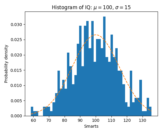
Note
In addition to the above described arguments, this function can take a data keyword argument. If such a data argument is given, the following arguments are replaced by data[<arg>]:
- All arguments with the following names: ‘weights’, ‘x’.
-
matplotlib.pyplot.hist2d(x, y, bins=10, range=None, normed=False, weights=None, cmin=None, cmax=None, hold=None, data=None, **kwargs)¶ Make a 2D histogram plot.
Parameters: x, y: array_like, shape (n, )
Input values
bins: [None | int | [int, int] | array_like | [array, array]]
The bin specification:
- If int, the number of bins for the two dimensions (nx=ny=bins).
- If [int, int], the number of bins in each dimension (nx, ny = bins).
- If array_like, the bin edges for the two dimensions (x_edges=y_edges=bins).
- If [array, array], the bin edges in each dimension (x_edges, y_edges = bins).
The default value is 10.
range : array_like shape(2, 2), optional, default: None
The leftmost and rightmost edges of the bins along each dimension (if not specified explicitly in the bins parameters): [[xmin, xmax], [ymin, ymax]]. All values outside of this range will be considered outliers and not tallied in the histogram.
normed : boolean, optional, default: False
Normalize histogram.
weights : array_like, shape (n, ), optional, default: None
An array of values w_i weighing each sample (x_i, y_i).
cmin : scalar, optional, default: None
All bins that has count less than cmin will not be displayed and these count values in the return value count histogram will also be set to nan upon return
cmax : scalar, optional, default: None
All bins that has count more than cmax will not be displayed (set to none before passing to imshow) and these count values in the return value count histogram will also be set to nan upon return
Returns: The return value is
(counts, xedges, yedges, Image).Other Parameters: cmap : {Colormap, string}, optional
A
matplotlib.colors.Colormapinstance. If not set, use rc settings.norm : Normalize, optional
A
matplotlib.colors.Normalizeinstance is used to scale luminance data to[0, 1]. If not set, defaults toNormalize().vmin/vmax : {None, scalar}, optional
Arguments passed to the
Normalizeinstance.alpha :
0 <= scalar <= 1orNone, optionalThe alpha blending value.
See also
hist- 1D histogram
Notes
Rendering the histogram with a logarithmic color scale is accomplished by passing a
colors.LogNorminstance to the norm keyword argument. Likewise, power-law normalization (similar in effect to gamma correction) can be accomplished withcolors.PowerNorm.Examples
(Source code, png, pdf)
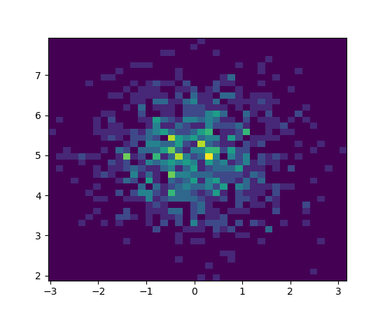
Note
In addition to the above described arguments, this function can take a data keyword argument. If such a data argument is given, the following arguments are replaced by data[<arg>]:
- All arguments with the following names: ‘weights’, ‘x’, ‘y’.
-
matplotlib.pyplot.hlines(y, xmin, xmax, colors='k', linestyles='solid', label='', hold=None, data=None, **kwargs)¶ Plot horizontal lines at each
yfromxmintoxmax.Parameters: y : scalar or sequence of scalar
y-indexes where to plot the lines.
xmin, xmax : scalar or 1D array_like
Respective beginning and end of each line. If scalars are provided, all lines will have same length.
colors : array_like of colors, optional, default: ‘k’
linestyles : [‘solid’ | ‘dashed’ | ‘dashdot’ | ‘dotted’], optional
label : string, optional, default: ‘’
Returns: lines :
LineCollectionOther Parameters: kwargs :
LineCollectionproperties.See also
vlines- vertical lines
Examples
(Source code, png, pdf)
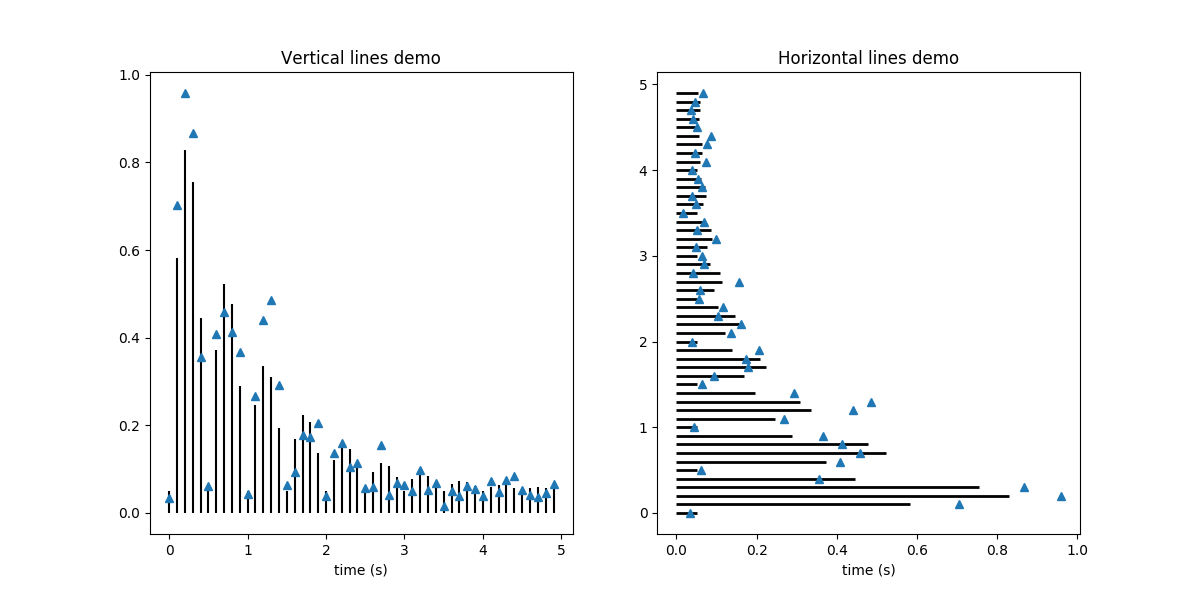
Note
In addition to the above described arguments, this function can take a data keyword argument. If such a data argument is given, the following arguments are replaced by data[<arg>]:
- All arguments with the following names: ‘xmax’, ‘xmin’, ‘y’.
-
matplotlib.pyplot.hold(b=None)¶ Deprecated since version 2.