The Risk-Neutral Closing Price, Behavioural Economics, Prospect Theory, and Nearly $5K in 3 Weeks?!

I’m gonna be honest… (and trying not to sound like a complete cornball at the same time) but this post should probably be behind a paywall. What’s discussed in this post has provided me with extreme edge the past few weeks, but, like all trading strategies, it comes with caveats, and in addition, like always, it probably can’t just be copy-traded. Your mileage may vary, so I’m posting it risk-free anyway. 😁 (pun definitely intended)

In short, I’m back into options - I was pulled into some 2% bonus offer by Robinhood and refunded my account back on October 30th (which I haven’t used since 2023) with just $1000… and have just short of 5x’d it in about 3 weeks…

People have been obsessing about timestamps recently, so here’s my monthly/annual P&L from Robinhood:

And all my bank statements, filtered for ‘robinhood’ in the past 60 days (the $5 transfer? - Yes, they suckered me into a month of gold as well 😂):

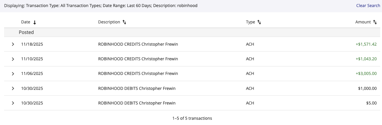
(For the wallstreetbets ‘positions or ban folks’, this was all made with a variety of QQQ puts over the past 3 weeks: I was in puts for both that ‘overnight surprise’ the Monday after FOMC week, and also during that 3-day balance break last week (3 days of MAE!), and subsequent 2% down day in equities. Finally, also I caught that big afternoon break to the downside on Monday this week (November 17th).) I journaled most of these trades in The Wheel Screener Discord - but no promise of how well I will keep up with that in the future. I’m trying, though!

Even then, in almost all of these trades, my performance could have been better. I am still struggling with closing too early (ringing in my ears constantly is TrAdInG iS nOt AbOuT BeInG RiGhT bUt MakInG mOnEy - which probably has cost me thousands over the years, and especially thousands in the past few weeks, but anyway, I’m getting off topic - all that individual psychology stuff is for another post at another time… also looking at you shrub, telling me to close out contracts at +100%!!! Some of those puts went 300%+ and beyond, wild markets…)

So anyway, what’s been helping me and giving me an extra edge recently? Let me introduce you to the work of Breeden & Litzenberg (1978) essentially states:

…the price of a $1.00 claim received at a future date, if the portfolio’s value is between two given levels at that time, is derived explicitly from a second partial derivative of its call option pricing function…

In other words, for a given options chain and given expiry, you can take the second derivative of all the call prices in that chain, and you’ll get the implied probability density function of the underlying’s ‘most likely’ closing price, in risk-neutral conditions.

A more technical flow looks like this. During regular trading hours, at any desired time period that fits your trading style (with 0-1DTEs, I find every 60 seconds is good enough for a poorboi retail trader like me), do the following:

1. Fetch all future expiry options chains for a given symbol from your data source of choice

2. Calculate the probability density function based on the work of Breeden & Litzenberg (Go code below on how to do this below - essentially it is the second derivative of call ) for each expiry.

3. For the 0DTE expiry options chain, note and track both the value and differences between spot and the median and mode
   

While trading, I find a few ways of looking at the data useful:

• The current ‘median’ or average price

• The current ‘most likely’ or mode price

• The difference of spot between the two

• The curves of the current and future expiry PDF curves

• The sum of all probabilities at each strike above and below the current spot

• … and working on many other exotic ways to interpret this data

As promised, here is what my go code looks like for deriving this PDF:

// EstimateImpliedProbabilityDistribution estimates an implied probability density
// function (PDF) for a single expiry using Breeden-Litzenberger style numerical
// differentiation of call prices across strikes. It also computes summary
// statistics such as mode (most likely), median, mean (expected value),
// expected move (stdev) and a basic tail skew metric.
//
// Parameters:
// - symbol: underlying ticker
// - description: descriptive string for the underlying
// - underlyingPrice: current spot/mark price of the underlying
// - callOptions: slice of call option contracts for a given expiry
// - mode: execution mode used for logging/notification decisions
//
// Returns an ImpliedProbabilityDistribution object populated with strike-level
// probabilities and top-level metrics, or an error if the distribution cannot
// be computed (for example, not enough strikes or zero mass).
func EstimateImpliedProbabilityDistribution(callOptions []types.Contract) (types.ImpliedProbabilityDistribution, error) {
	// ensure that callOptions are sorted by strike price, ascending
	sort.Slice(callOptions, func(i, j int) bool { return callOptions[i].Strike < callOptions[j].Strike })
	n := len(callOptions)
	if n < 3 {
		return types.ImpliedProbabilityDistribution{}, fmt.Errorf(”not enough data points”)
	}
	// get expiration from first option (assuming all same expiry)
	expiryDate := callOptions[0].ExpirationDate.UnixMilli()
	// Estimate second derivative numerically (central difference)
	strikeProbabilities := make([]types.StrikeProbability, n)
	for i := 1; i < n-1; i++ {
		kPrev := callOptions[i-1].Strike
		kNext := callOptions[i+1].Strike
		kCurr := callOptions[i].Strike
		midPrev := (callOptions[i-1].Bid + callOptions[i-1].Ask) / 2
		midCurr := (callOptions[i].Bid + callOptions[i].Ask) / 2
		midNext := (callOptions[i+1].Bid + callOptions[i+1].Ask) / 2
		cPrev := midPrev
		cNext := midNext
		// Protect against division by zero if strikes are too close together
		strikeDiff := kNext - kPrev
		if math.Abs(strikeDiff) < 1e-9 {
			strikeProbabilities[i] = types.StrikeProbability{Strike: kCurr, Probability: 0}
			continue
		}
		d2 := (cNext - 2*midCurr + cPrev) / math.Pow(strikeDiff, 2)
		// f(K) = e^{rT} * d2C/dK2, ignoring discount for simplicity
		strikeProbabilities[i] = types.StrikeProbability{Strike: kCurr, Probability: math.Max(d2, 0)}
	}
	// Normalize densities to sum to 1
	sum := 0.0
	for _, d := range strikeProbabilities {
		sum += d.Probability
	}
	// Protect against division by zero if all probabilities are 0 or negative
	if sum < 1e-9 {
		return types.ImpliedProbabilityDistribution{}, fmt.Errorf(”insufficient probability mass to normalize (sum=%f)”, sum)
	}
	for i := range strikeProbabilities {
		strikeProbabilities[i].Probability /= sum
	}
	// Compute summary stats
	// most likely price (mode)
	mostLikelyPrice := strikeProbabilities[0].Strike
	maxProb := 0.0
	for _, d := range strikeProbabilities {
		if d.Probability > maxProb {
			maxProb = d.Probability
			mostLikelyPrice = d.Strike
		}
	}
	// Compute cumulative distribution for median & tails
	cumulative := 0.0
	median := strikeProbabilities[len(strikeProbabilities)/2].Strike
	for _, d := range strikeProbabilities {
		cumulative += d.Probability
		if cumulative >= 0.5 {
			median = d.Strike
			break
		}
	}
	// Expected value, variance, and expected move
	mean := 0.0
	for _, d := range strikeProbabilities {
		mean += d.Strike * d.Probability
	}
	variance := 0.0
	for _, d := range strikeProbabilities {
		diff := d.Strike - mean
		variance += diff * diff * d.Probability
	}
	expectedMove := math.Sqrt(variance)
	// Tail skew: rightTail / leftTail relative to mean
	leftTail, rightTail := 0.0, 0.0
	for _, d := range strikeProbabilities {
		if d.Strike < mean {
			leftTail += d.Probability
		} else {
			rightTail += d.Probability
		}
	}
	tailSkew := rightTail / math.Max(leftTail, 1e-9)
	// Calculate cumulative probabilities above and below spot price
	cumulativeBelowSpot := 0.0
	cumulativeAboveSpot := 0.0
	for _, d := range strikeProbabilities {
		if d.Strike < underlyingPrice {
			cumulativeBelowSpot += d.Probability
		} else if d.Strike > underlyingPrice {
			cumulativeAboveSpot += d.Probability
		}
	}
          // do whatever you'd like with the curves or statistics
}

Remember that these numbers reflect the risk-neutral closing price only! Do not get them confused with the current target price! With that said… do these curves and numbers predict price perfectly? Also, no - sorry if you were looking for the holy grail (I’m still looking too!), however, watching these numbers over the past few weeks of trading, I can say they do provide an edge - at least for my trading style with 1-4DTE options!

Since this reflects the risk-neutral price, it will always be below the spot, since there is always a premium payed for downside protection.

To summarize, the signal I’m starting to form is something like this:

Difference between spot and median price is -20 to -30: strong potential bearish bias

Difference between spot and median price is -10 to -20: standard risk hedging, no bias

Difference between spot and median price is 0 to -10: market not paying for nearly any, if at all downside hedges, bullish bias

This process and signal is about as new to me as it probably is to you - so your mileage may vary!

Like any other signal or model, what we can do is use these numbers to make educated bets. For example, on QQQ, which is the symbol I trade exclusively, even during the 3 days consolidation November 10-12th, the median price was stubbornly and continually reported at 585 (yes, I know, way below the 617-625 range we were seeing!) This information, along with the continued rejections around the 623-625 area, as well as some backtesting on globex gaps (maybe yet another post for another time) helped me build conviction on my short position.

And remember Friday the 7th? which was a deep sell and then “V” shaped recovery? Even after the steep sell in the morning, we sort of bottomed around 600. Here’s a plot of what the risk-neutral price was calculated at near-minute intervals (sorry for the time discontinuities too - still polishing the system)

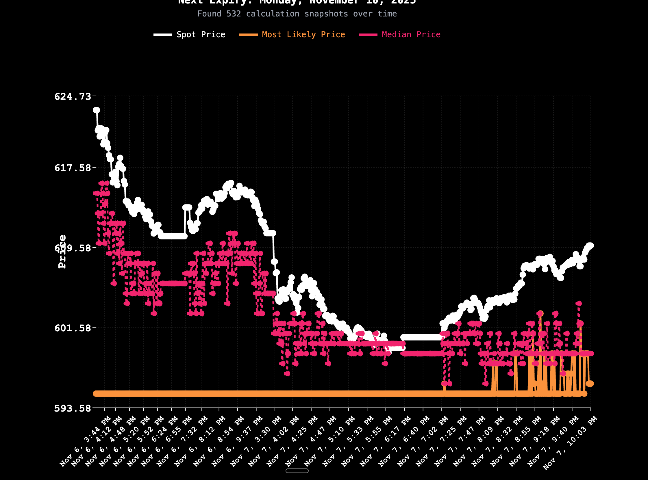
Note that the spot price comes down to the risk-neutral close price… chops around, and then we revert higher. Notice that even the most likely price begins to show spikes to the upside. I interpreted it as “market participants are not budging or otherwise don’t see a need to hedge any lower this session”. This bounce from 600 in the Q’s subsequently printed 20, or even 25 points into the following week - if you were patient!

Here’s where the risk-neutral closing price idea gets interesting: what if we can use the logical fallacies of market participants (especially retail, sorry guys) to better scale the risk-neutral closing price, to make it more simply ‘actual closing price’. Specifically, I’m talking about loss aversion within prospect theory, which more or less states that most people, on average, are more averse to loss than they are to a gain of equal size. (and both

Tabulated, the famous formula from Kahneman & Tversky, 1979, is:

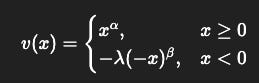
Where the value of any gain (x >= 0) diminishes with 0.88, as well as any loss (x < 0) diminishes with 0.88, BUT losses are penalized with an additional -2.25 multiplier (λ). This is the loss aversion factor! So, if we can scale what we assume is the ‘max downside target’ i.e. the risk-neutral closing price, by this model including loss aversion values… well, you can get the idea of where I’m going with this pricing model 😉

(Btw - I really thought I was being the first brilliant thinker to apply human psychology to market prices, turns out I’m waaaaay behind - all sorts of institutions and algos are already using these concepts - I should have guessed, nothing new under the sun 😉)

Still, for retail, I think it’s a pretty good direction to start thinking about.

Single-time snapshots for these PDF calculations are behind the premium tier over at my newest FinTech product, VannaCharm. Currently, it is based on options chains data from the previous close, but we’re looking to work with some brokers to allow individuals to use our platform to have these calculated live in real time on the VannaCharm platform. (as I’ve been doing privately with my broker feeds the past few weeks).

It’s funny that I was always interested in human psychology but it took me so long to realize that all the ‘trader psychology’ is really nothing more than plain ol’ general human psychology. This may be one of the reasons I fell in love with markets subconsciously in the first place, since they are really one in the same. Trends, patterns, and themes I’ve been interested in for years, I can finally see in a clearer lens as all being related.

It’s finally all coming together.

Thanks to these authors:

Ezhu for his study of the work of Breeden & Litzenberger with a trading strategy:
https://medium.com/@ezhu1009/on-the-predictive-power-of-breeden-litzenbergers-risk-neutral-distribution-d6ad63c9db41

Robert Martin for his super clear and step-by-step explanation on option implied probability density functions (truly well written, I strongly advise anyone intersted in risk-neutral :

https://reasonabledeviations.com/2020/10/01/option-implied-pdfs/

https://reasonabledeviations.com/2020/10/10/option-implied-pdfs-2/

As mentioned in this article, these risk-neutral probability density functions (and various ways to view them) are part of a premium subscription on vannacharm.com

I’m finding this whole new world of behavioural economics fascinating and will be publishing a lot of new work and metrics over there in the months to come. I hope you’ll consider subscribing.

As always, thanks for stopping by and good luck out there in these crazy markets!

-Chris