Scaling Laws: The Law Behind Every LLM — Kaplan vs. Chinchilla vs. Inference-Optimal (2020-2026)

For decades, this curve was blueprint of deep learning. If your model is too simple (relative to the complexity of the task), it underfits, it can’t capture the pattern. Increasing the complexity of the model usually led to better results, but if you keep pushing the complexity up on a fixed dataset, then something worse happens: error stops falling and starts climbing again. The model isn’t learning anymore. It’s memorizing noise (overfitting).

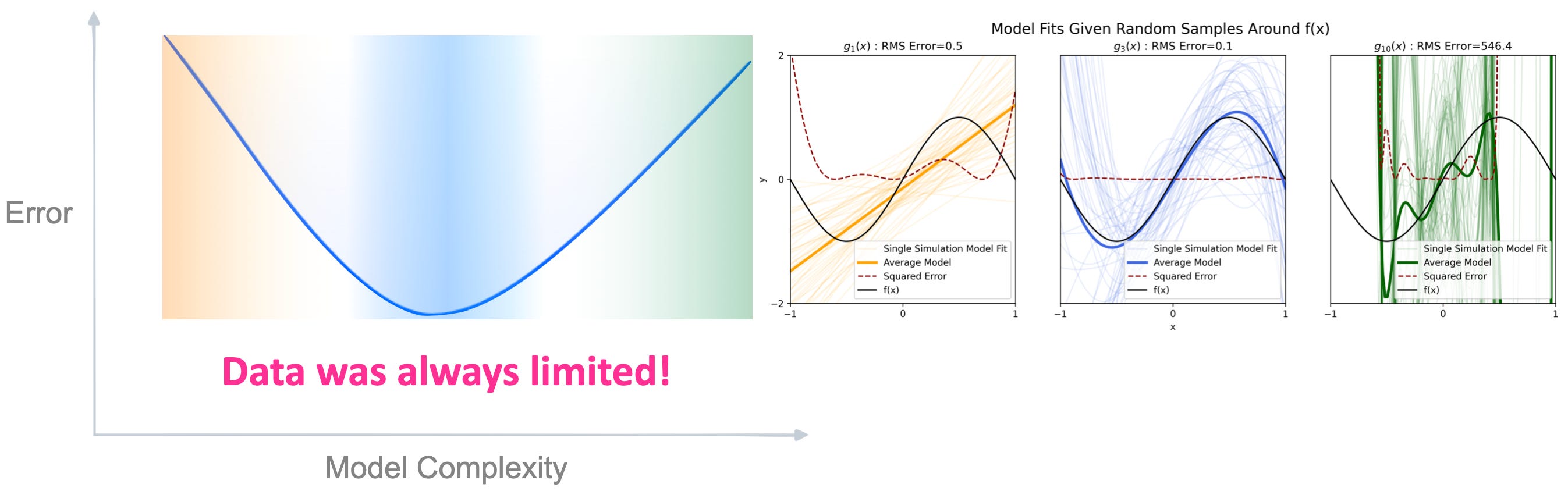
That second half of the curve is the one that mattered. It’s why “just make the model bigger” used to be bad advice, not good advice. And it wasn’t really a modeling problem. It was a supply problem.

Data was always limited. Every gain in model capacity ran straight into the cost of labeling more of it. Human annotation is slow, expensive, and does not scale linearly with your ambition. For decades, that constraint (not compute nor the architecture) was the actual bottleneck on how good a model could get.

The wall didn’t move until someone stopped asking humans to label the data at all.

Self-supervision is the trick: use the text itself as the label. Predict the next word. “The cat sat on the ___” and the answer, “mat,” was sitting right there in the training corpus the whole time. No annotator required. Every book, every codebase, every web page instantly became labeled data, for free.

That single move deleted the data bottleneck. Suddenly the constraint on how good a model could get wasn’t how much labeled data existed. It was how much compute you were willing to spend processing it. The bias-variance wall didn’t get solved. It got sidestepped, by making the “not enough labeled data” side of the curve functionally irrelevant.

Which immediately created a new problem: if data is no longer scarce, and compute is the only real constraint, how do you decide where a bigger compute budget actually goes?

The Equation Behind Every Training Run

Every training run has a cost, measured in FLOPs, and it comes down to a deceptively simple formula:

C ≈ 6 × N × D

N is parameter count. D is dataset size in tokens. The 6 is fixed, we need 2 FLOPs for the forward pass, and 4 for the backward pass, per parameter, per token. You don’t get to negotiate this. The only lever you control is how you split your budget between N and D.

That fundamental allocation question, bigger model or more data, has been answered three different ways in five years, and each answer produced a visibly different generation of models.

In 2020, OpenAI’s Kaplan et al. modeled loss as a function of N and D independently and found something that looked decisive: the exponent on parameters was small enough that scaling the model mattered far more than scaling the data. Their math said that for every unit of new compute, roughly 73% should go into making the model bigger, and only 27% into feeding it more text.

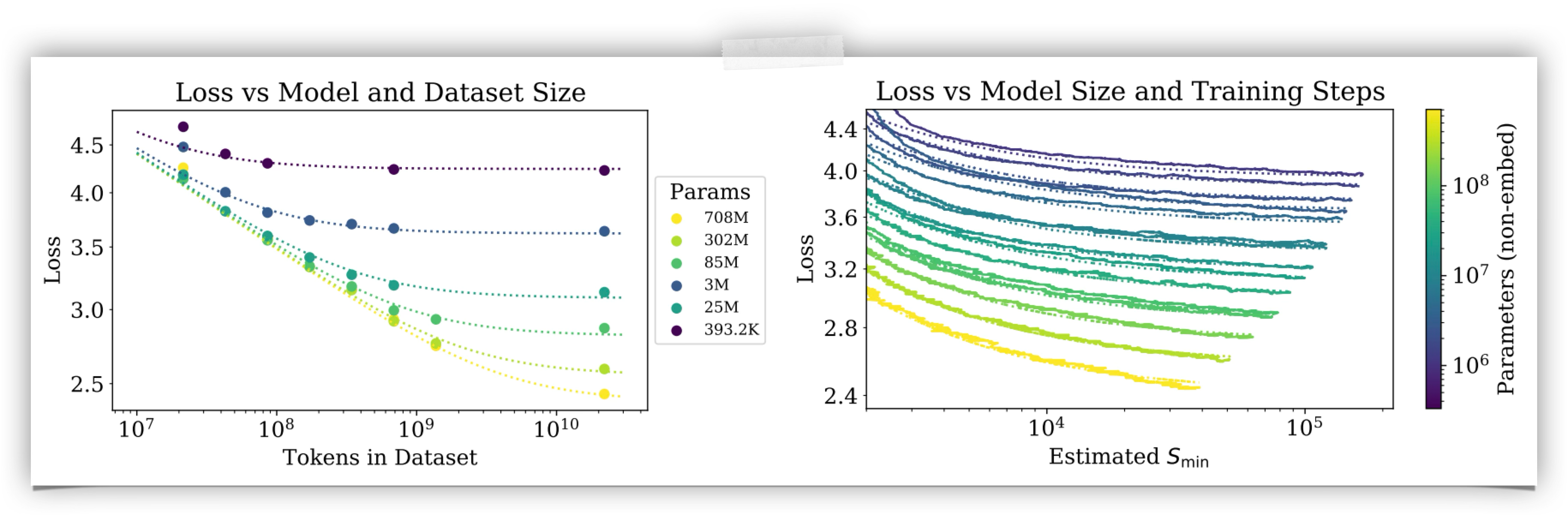
Look at the left panel: every parameter count eventually flattens out, hitting a data ceiling regardless of how much more text you feed it. That flattening is exactly what told Kaplan et al. that parameters, not tokens, were the lever worth pulling.

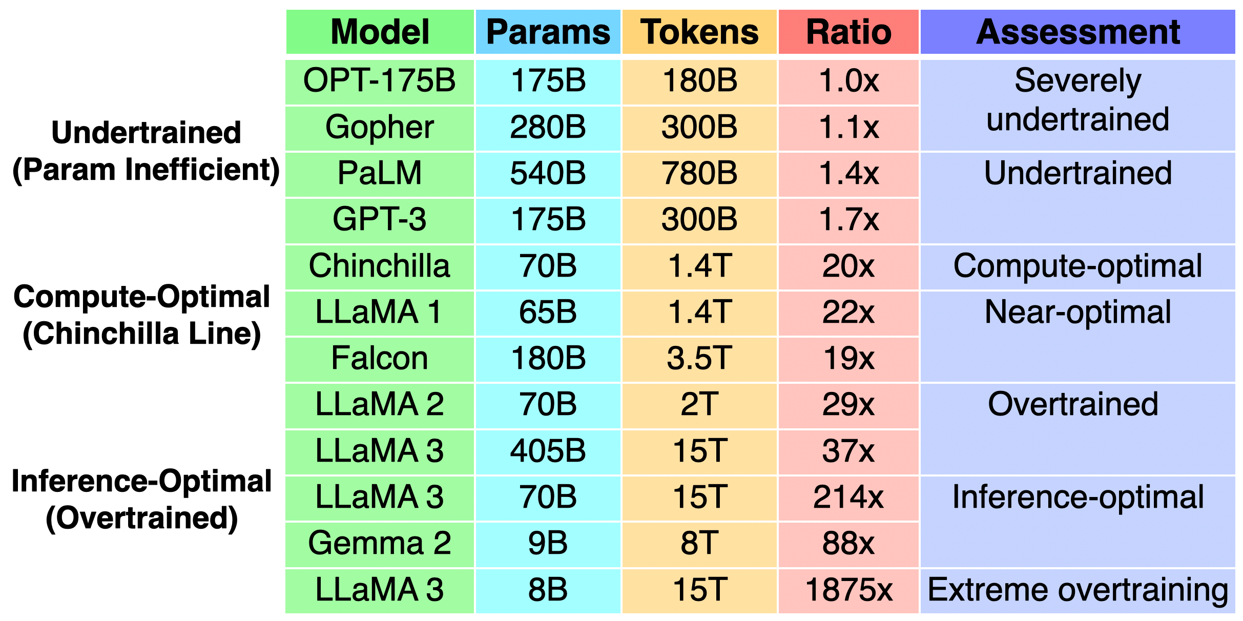
Labs took that seriously. GPT-3 landed at 175B parameters trained on 300B tokens. PaLM went to 540B parameters on 780B tokens. That’s a token-per-parameter ratio under 2x on both — models with enormous capacity and comparatively little to actually learn from.

The cost is that “bigger” and “smarter” quietly stopped meaning the same thing. A model can have hundreds of billions of parameters and still be undertrained, plenty of room to memorize, not enough signal to fill it. Kaplan’s numbers weren’t wrong about the trend. They were wrong about the destination.

Note: the gap wasn’t a math error so much as a methodology one. Kaplan’s fits excluded embedding parameters, were built mostly on smaller models, and used fixed learning-rate schedules that penalized runs with more data, all of which quietly tilted the conclusion toward “make it bigger.” Get your fitting methodology wrong at this level and the entire first generation of frontier models inherits the bias.

Two years later, DeepMind’s Hoffmann et al. re-ran the experiment properly, over 400 models, tuned learning-rate schedules, IsoFLOP contours instead of single-variable fits. Their model of loss added a parameter-bound term and a data-bound term together instead of treating them as separate stories, and the two exponents came out almost identical.

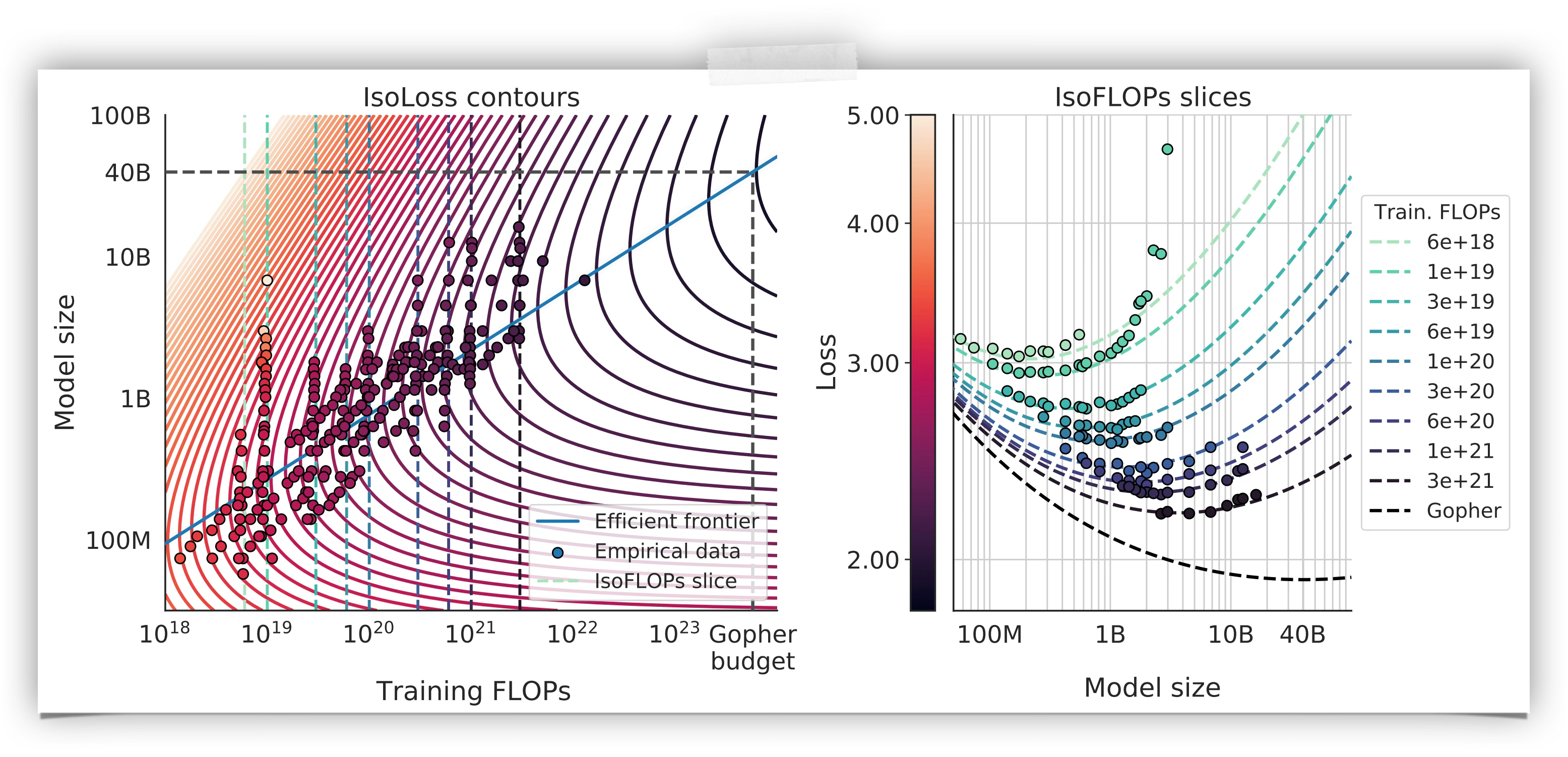
That efficient frontier line running through the contours on the left is the whole paper in one stroke. For any fixed compute budget, there is one model size that sits at the bottom of the curve on the right, not the biggest model you can afford, the one that minimizes loss for that exact budget.

Translation: parameters and data matter equally. Their rule of thumb, roughly 20 tokens per parameter, became the compute-optimal line. Chinchilla, at 70B parameters trained on 1.4T tokens, outperformed GPT-3’s 175B outright. Not because it was bigger. Because it wasn’t starved.

The cost is that “compute-optimal” only optimizes for one thing: the training run itself. Chinchilla tells you the cheapest way to reach a given loss. It says nothing about what happens after training ends, and after training ends is where a deployed model actually lives.

Here’s the question Chinchilla never had to answer: what if the model gets called a billion times after you finish training it?

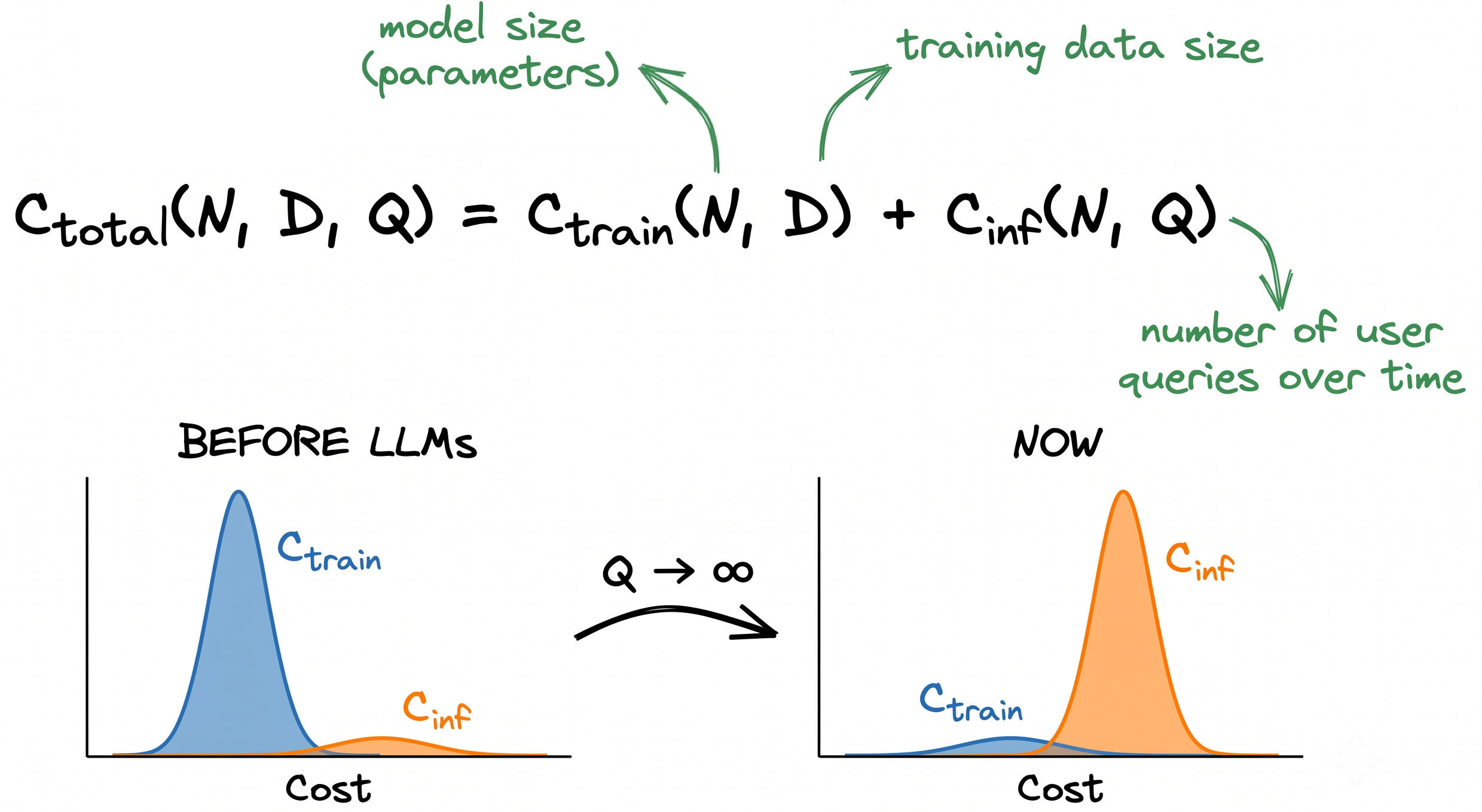
Total cost isn’t just training cost. It’s:

Q is the number of queries the model serves over its lifetime. Training cost is a one-time invoice. Inference cost is multiplied by every single call the model ever answers, and it scales directly with N. Every extra parameter you’re compute-optimal about at training time is a parameter you pay for again, and again, on every request, forever.

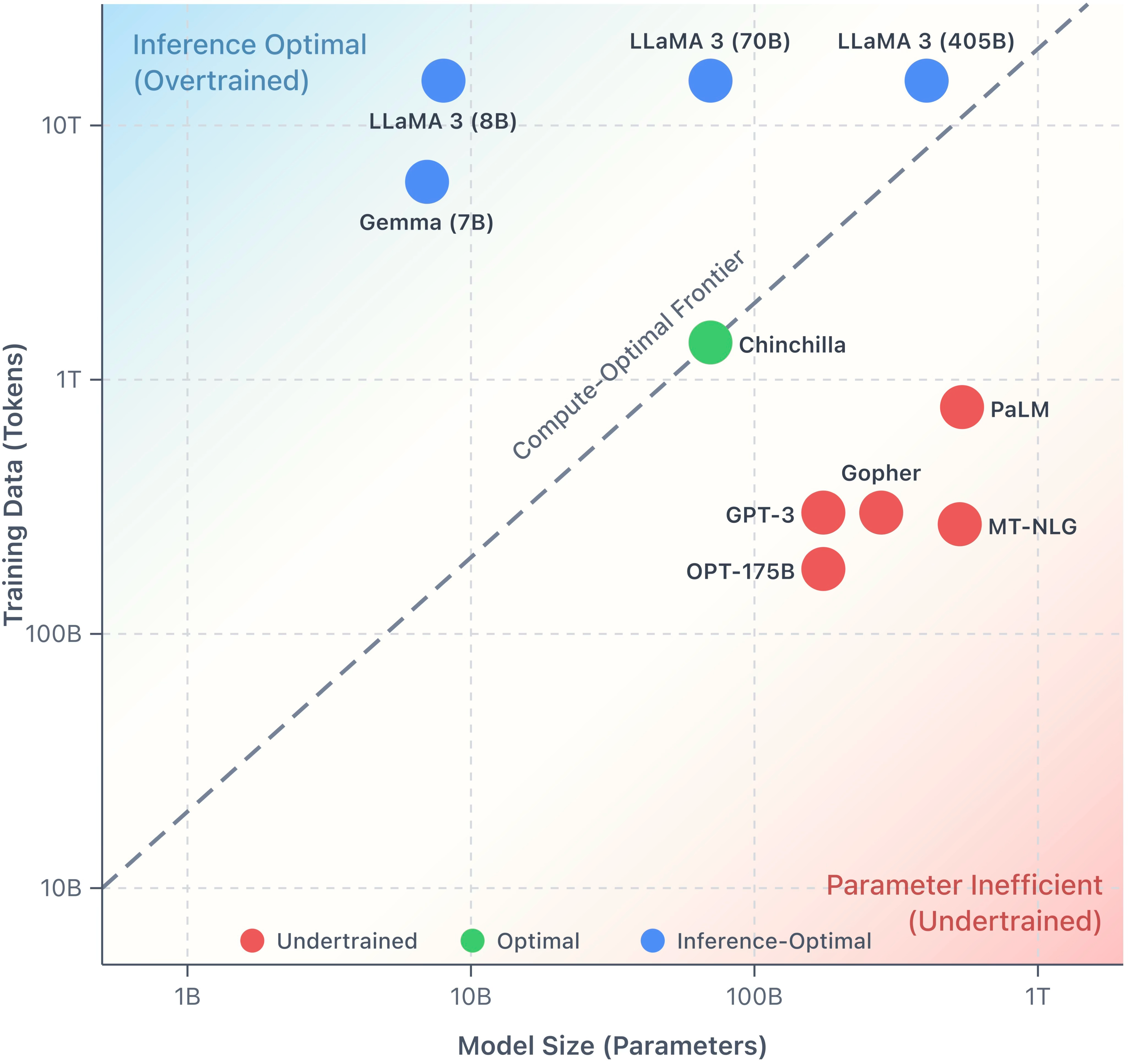
That top-left region is where production actually lives now. Chinchilla sits exactly on the frontier line, right where the math says it should. LLaMA 3 8B and Gemma sit nowhere near it, they’re pushed far above the “optimal” line, trained on far more tokens than their parameter count calls for. That’s not a mistake on the chart. That’s the whole strategy.

Once a model is deployed at real scale, Q dominates. This is the whole reason modern labs deliberately overtrain. LLaMA 3 8B was trained on 15 trillion tokens, a ratio of roughly 1,875 tokens per parameter, nearly a hundred times past the Chinchilla line. That’s not a training mistake. It’s a trade: eat a larger, one-time training bill to shrink N, so that every one of the billions of queries that follow is cheaper, faster, and lighter to serve.

The cost is real, it’s just paid by a different line item. You spend more up front, on purpose, to make the recurring bill smaller. For a company serving a chat app to millions of users, that trade is obvious. For anyone running agentic pipelines, where a single user request can fan out into dozens of model calls across specialized agents, it’s not optional. Q isn’t a hypothetical variable in that formula. It’s your architecture.

Note: this is also where a chunk of the “emergent capability” story gets less mystical than it looks. Skills like in-context learning and chain-of-thought used to show up only past the 100B-parameter mark. Overtraining smaller models on enormous, high-quality datasets has leaked a lot of that same behavior into far smaller footprints. Scale didn’t get less important. It got redistributed, from parameters into tokens.

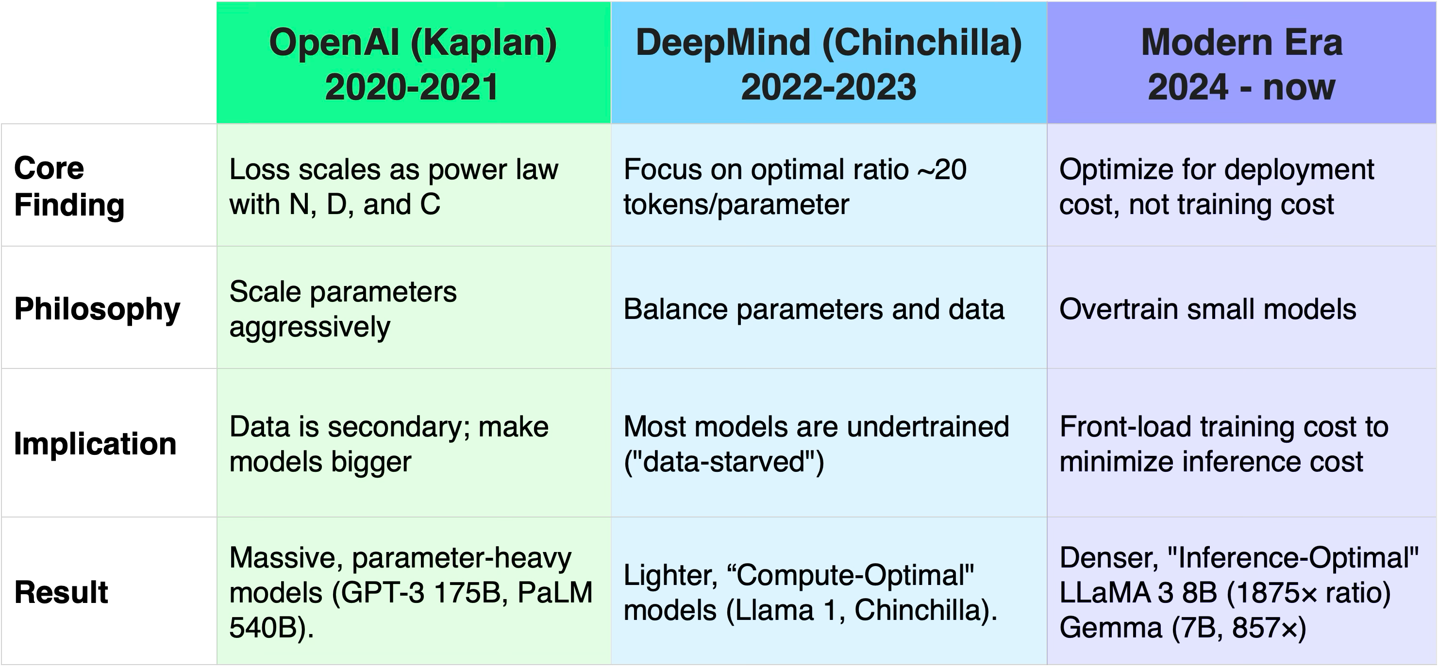
Same compute equation. Three completely different answers about where the money goes — and each one produced models you’d recognize immediately.

The Dose Verdict

Scaling laws were never a fixed law of physics. They’re a snapshot of who’s paying, and when. The bias-variance wall was a data-supply problem, solved by treating text as its own label. Kaplan optimized for a world where data was assumed scarce even after that fix. Chinchilla optimized for the cheapest possible training run. Neither one asked what happens when the model ships and Q stops being a variable in a paper and starts being your traffic.

If you’re building agentic systems, that’s the only question that matters. The rule of thumb for picking a model in an agentic stack is “what was this model overtrained for, and does that match how many times I’m about to call it.” You are the Q in that equation. Choose accordingly.

Until next dose — Dr. Ryan Rad